Optimal Event Handling by Multiple UAVs

(1)

Optimal Event Handling by

Multiple UAVs

M. (Martijn) de Roo

MSc Report

Committee:

Prof.dr.ir S. Stramigioli

Dr. R. Carloni

Dr. P. Frasca

Dr. W.S. Rossi

July 2015

(2)

(3)

(4)

iv MSC REPORT, JULY 2015

PREFACE

This MSc report in front of you is the result of a graduation project at the research group Robotics and Mechatronics of the University of Twente.

Several persons have contributed both academically and practically to this thesis, I am very thankful to them.

“

text

The most exciting phrase to hear in science, the one that heralds new discoveries, is not ’Eureka!’, but ’That’s funny ...’

- Isaac Asimov

”

(5)

ROO, DEet al.: OPTIMAL EVENT HANDLING BY MULTIPLE UAVS v

CONTENTS

I Introduction 1

I-A Group System . . . 1

I-B Individual System . . . 1

II Control Architecture 2 III Group System 2 III-A Optimal coverage problem . . . 2

III-B Gradient descent optimization . . . 3

III-C Implementation of the control law . . . 4

IV Individual System 4 IV-A UAV . . . 4

IV-B Path planning . . . 5

IV-C Controller . . . 6

IV-C1 Position control . . . 6

IV-C2 Path following . . . 6

IV-D Collision avoidance . . . 7

V Simulations 7 V-A Hardware . . . 7

V-B Results 20-sim . . . 8

V-C Results ROS . . . 8

V-D Results MATLAB . . . 9

VI Experiments 9 VI-A Hardware . . . 9

VI-B Results . . . 10

VII Conclusion 11 VIII Recommendations 11 Appendix A: Algorithm group system 12 Appendix B: Generalization Metric Manifold 14 B-A Gradient descent optimization . . . 14

Appendix C: Path Following 14 C-A Radius . . . 14

C-B Error radius . . . 14

C-C Line of sight . . . 16

C-D Curvature based path following . . . 16

Appendix D: Circumcircle calculation 17 Appendix E: Manual 17 E-A Prerequisites . . . 17

E-B Installation . . . 18

E-C Usage . . . 18

(6)

(7)

MSC REPORT, JULY 2015 1

Optimal Event Handling by Multiple UAVs

Martijn de Roo, Paolo Frasca, and Raffaella Carloni

Abstract—In this paper a control architecture is presented, designed for event handling by a UAV (Unmanned Aerial Vehicle) network with an optimal approach. The architecture allows the calculations for the placement of UAVs in an area for tasks that need to be served by more than one UAV at the same time. The feasibility of this method is shown in simulations and is made ready for a test setup consisting out of several quadcopters.

Index Terms—UAV, quadcopters.

I. INTRODUCTION

E

VENT handling can be important, depending on the nature of the events. An example of this is the SHERPA project [1], which aims to develop a robotic platform with UAVs and ground robots to support search and rescue ac-tivities. Being able to manage these activities as optimal as possible is of high interest, because it will offer the possibility to save time in situations where time is not enough. Four subtopics are identified that combined can achieve optimal event handling: (1) optimal control of the UAVs, (2) achieving optimal paths through an area, (3) optimal coverage of an area such that UAVs are placed in positions where they can serve the most events, (4) optimal event handling such that events can be serviced as fast as possible, with the main focus being on the optimal coverage.

The contribution that will be delivered is a system that calculates the position of the UAVs based on where events are likely to occur and rearranges the positions of the UAVs to meet this coverage, allowing the response of UAVs to events. We continue by splitting our approach, one part directed at the coverage and event handling, which effects all UAVs, the Group System, and the other part directed to control and paths, theIndividual System.

A. Group System

The group system delivers the distribution of the UAVs and selects which UAV goes where. The coverage of an area by UAVs needs to be solved; ideally the solution takes in account a certain probability distribution of events occurring in an area and the possibility of requiring more than one UAV for an event. The dynamic property of the UAV makes the problem rather complicated and does not add much merit under the assumption that the UAV has a sufficient fast turning rate, like a quadcopter. A common solution to the coverage problem are Voronoi tessellations [2]–[4]. Voronoi tessellations divide space in a number of regions based on an set of generators,

This work has been partially funded by the European Commission’s Seventh Framework Programme as part of the project SHERPA under grant no. 600958. The authors are with the Faculty of Electrical Engi-neering, Mathematics and Computer Science, CTIT Institute, University of Twente, The Netherlands. Email: [email protected], {p.frasca, r.carloni}@utwente.nl.

on which the resulting regions give the area for which that generator is closer than any other generator. While this works in Euclidean space, it is harder to achieve in non-convex space, as argued in [3], which gives a solution to the non-convex Voronoi problem by discretizing it and solving it with Lloyd’s algorithm. The downside of this is that the problem can be a computationally heavy approach to solve. The distribution of UAVs can be solved offline if the amount of UAVs and geography is known, so in some applications computational heavy solutions are allowed.

While the research in [3] is of interest for us, it does not cover for the possibility of requiring more than one UAV for an event, thus it will be extended for multiple density functions that depend on the amount of required UAVs.

The other part of the group system is the selection of which UAV has to go where. Ideally the time required for an event is known and new events near the currently occupied UAV might be able to be processed faster by waiting for the occupied UAV to finish. This is a rather extended topic but might be interesting for extending the framework. The time for an event is assumed to be unknown, therefore no sequential events are considered and the system will work on a first come first served process.

For the selection of the UAV that has to respond to the appearance of an event, the path planning can be used; by calculating for each UAV the length of the path to the event and taking the shortest one of them, the UAV can be selected that has to go. For this it is assumed that the longer the distance is, the more time it takes before an event can be serviced.

B. Individual System

The individual system manages the movement of the UAV and ensures that no collisions occur. Ideally a solution is used that is able to take in account all the UAVs at the same time, takes in account the paths they follow and avoids possible collisions beforehand by changing the paths they follow. A decentralized approach for this is used, otherwise one central configuration has to be solved, which is a NP-complete problem [5] and is hard to solve in real-time.

Because the system is decoupled, the path planning will be done separately from the control action, which means that separate obstacle avoidance is required. As the chance of a collision occurring is rather small, because UAVs will tend to serve events close to them, it might only be useful in close spaces.

(8)

2 MSC REPORT, JULY 2015

The individual system will be addressed with the following individual topics: control, path planning and collision avoid-ance.

II. CONTROLARCHITECTURE

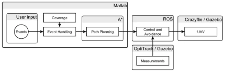
An overview of the control architecture is shown in Fig. 1. The architecture consists of anIndividual Systemand aGroup System that act based onEvents.

TheGroup Systemdetermines which UAV goes where, the Coverage module determines the placement of the UAV(s) based on the area and a density function for each amount of UAV(s) that is needed for events in the area, the Event handling module determines which UAV(s) is(are) closest to the event and then forwards the event location to theIndividual System of the UAV(s).

The Individual system takes the UAV from its original position to the position of the event. The Path Planning module determines the path that needs to be travelled and takes into account the area, theControl and Avoidancemodule then applies a control on the path to make sure that it is followed as close as possible, without collisions occurring with other objects. The output of the Control and Avoidance module is sent to the UAV to control it.

Fig. 1. Control Architecture, shows the global overview of the system on how events are handled, first by the group system, and then by the individual system.

III. GROUPSYSTEM

The goal of the group system is to optimally assign UAVs to the events. In our system, optimality is defined as minimizing the average waiting time incurred by the events. This goal is achieved by deploying the group of UAVs in an optimal configuration (via the Coverage module) and by assigning, upon the appearance of an event, the closest UAVs to service it (via the Event handling module). The key part here is optimizing the configuration (i.e., the positions) of the UAVs while they wait for the appearance of the events. In this section, we provide the formal description and a solution for this optimization problem.

A. Optimal coverage problem

Let Ω be a bounded connected domain of RN, where in

our applications N ∈ {1,2,3}. In this domain, events take place according to a random spatial process. The events are heterogeneous in nature and thus require different numbers of UAVs to be serviced: consequently, we define for each

m∈ {1, . . . , M} a smooth density function φm: Ω→R>0,

representing at each point inΩthe density of events requiring

m UAVs. Let p ∈ Ωn _{be the vector of the UAV positions,}

where the position of the ith _{UAV is given by} _pi _{and let} ||q−pi|| denote the Euclidean distance between pi and a generic point q inΩ. For the sake of generality and in order to account for heterogeneities among the UAVs in terms of speed, we define for each i ∈ {1, . . . , n} a smooth strictly increasing convex function fi : _R_≥₀ → R≥0: consequently, fi(||pi−q||)will represent the travelling time of UAVifrom its current position to q. Whenever mUAVs are required by an event, we assume that the event cannot be serviced until it has been reached by all mUAVs: hence, the waiting time of the event is the travelling time of its m-th closest UAV. To formalize this fact, we shall write m-minS to denote the

m-th smallest element in a finite set of real numbersS. With this notation in place, we are ready to define the following integral cost function, which represents the expected service time of an event,

Jexp(p) = M X

m=1 Z

Ω

m-min

i∈{1,...,n}fi(||q−pi||)φm(q) dq (1)

and the corresponding optimization problem

min

p∈ΩnJexp(p).

In the special case when M = 1, this problem boils down to optimizing

Z

Ω min

i∈{1,...,n}fi(||q−pi||)φ(q) dq,

which is extensively studied for instance in [9] with the use of Voronoi tessellations of the domain Ω. In fact, also the cost (1) can be conveniently rewritten by using a suitable decomposition ofΩinto sub regions, in the following way:

LetW be a collection of subsets ofΩsuch that each region

Wm

i is indexed byi ∈ {1, . . . , n} andm∈ {1, . . . , M} and

for eachmthe sub-collection{Wm

i }i∈{1,...,n}is atessellation of Ω: that is,∪n

i=1Wim= Ω for everym andWim∩Wjm is

a set of measure zero ifi6=j. Note that the regionsWm

i are

not assumed to be connected, i.e., a region can consist out of several disjoint sub-regions. Given such a collection W, we can define the cost

J(p, W) =

n X

i=1 M X

m=1 Z

Wm

i

fi(||q−pi||)φm(q) dq. (2)

Writing this cost, we take each UAV i as responsible for servicing events in the region ∪mWm

i : in regionWi1 it shall

service all events, in regionW2

i it shall service all events that

require at least two UAVs, and so forth.

In order to link this generic cost with the expected cost (1) we need to define one specific collectionZ. Given a configu-rationpwith no coincident positions, let us then define the re-gionZm

i as the region ofΩsuch thatiis themthclosest UAV

to the points inZm

i . More formally, letZim={q∈Ω :∃H⊂ {1. . . n}such that|H|=m−1, i6∈H andfh(||q−ph||)≤ fi(||q−pi||)≤f`(||q−p`||)for allh∈ H, ` /∈H, `6=i}. Note that the sub-collection{Z1

(9)

ROO, DEet al.: OPTIMAL EVENT HANDLING BY MULTIPLE UAVS 3

Fig. 2. Example of the construction of the regions Zm

i with n= 3and

m= 2.

By virtue of its definition, Z minimizes J(p, W) as a function of W for fixed p. In fact, we have

Jexp(p) =J(p, Z) = min

W J(p, W)

for every p /∈ C, whereC ={p∈ Ωn : ∃i, js.t.pi =pj}.

This fact also permits to show –along the lines of [9, Theo-rem 2.16]– that the functionJexpis Lipschitz continuous on

its domain and continuously differentiable outside the set of coincident configurationsC.

Constructing the regions Zm

i : For the sake of clarity and

concreteness, we now illustrate with the help of Fig. 2 how to construct such regionsZm

i for an example with n= 3and m = 2. First, we construct the Voronoi regions Z1

i for each i. Next, to get the second closest tessellation of the Voronoi regionZ1

i, we leave out UAVifrom the generators and

con-struct the Voronoi tessellation generated by{1, . . . , n} \ {i}, which we denote Xi

k; note that ∪k6=iXki = Ω. By taking the

intersection of the new regionsXki and the regionsZi1for all iwe getT_k2,i=Z1

i ∩Xki. Finally, we define Zk2=∪iT 2,i k .

The same process can be repeated for the m = 3 case using the regions T_k2,i as the starting point. Special care has to be taken to make sure that, for the creation ofXk

j we not

only leave out k, but also the generators of all the parent tessellationsT_k2,i is based on, in this case only i, this is also why we cannot use Z2

k because it is based on two different

values of i. We give a more formal definition for the set of generators to also allow higher values ofm,{1, . . . , n}\({k}∪ K), whereK={all j for whichT_km,i∩Zl

j 6=∅ ∀l < m−1}.

B. Gradient descent optimization

The minimization of the coverage function can be sought by following its gradient by the dynamics

˙

pk =−κ∂J(P)

∂pk ∀i∈ {1, . . . , n}, (3)

whereκ≥0. However, the coverage function is not convex, so a gradient descent will not in general reach a global minimum. We shall now compute the gradient under the simplifying assumption thatfi(x) =x2_{: this assumption, according to [3],}

is often adequate in practice and can be relaxed at the cost of more involved notation. We then have

∂J(P)

∂pk = ∂ ∂pk M X m=1 n X i=1 Z Zm i

||pi−q||2φm(q) dq (4a)

= M X m=1 n X i=1 Z Zm i ∂

∂pk||pi−q||

2_φm_{(q) dq} _(4b)

= 2 M X m=1 n X i=1 Z Zm i

||pi−q|| ∂

∂pk||pi−q||φm(q) dq

(4c) = 2 M X m=1 Z Zm k

||pk−q|| ∂

∂pk||pk−q||φm(q) dq,

(4d)

where for step (4a) to (4b) it is allowed to take the deriva-tive under the integral according to [4, Proposition 2] and for step (4c) to (4d) the summation is removed because

∂

∂pk||pi−q|| = 0, ∀k 6= i. Since

∂

∂pi||pi−q|| =

pi−q

||pi−q||,

Equation (3) becomes

˙

pi=−2κ M X m=1 Z Zm i

(pi−q)φm(q) dq (5)

which corresponds to steering each UAV towards a weighted “centre of mass” of its own responsibility region ∪mZm

i .

Since the change in the objective function

dJ(p(t))

dt =

n X

i=1

∂J(p(t))

∂pi pi˙ =−κ

n X

i=1

∂J(p(t)) ∂pi

2

is negative semidefinite and the trajectories p(t) stay in the bounded set Ωn_{, we are in the position to apply a LaSalle}

invariance principle to prove convergence to the critical points ofJ(p). Actually, special care must be taken becauseJ(p)

is not continuously differentiable in C, hence the LaSalle principle should be applied in the set Ωn \ C, which is not closed and is dense in Ωn. By using the generalized invariance principle in [9, E1.8], we thus obtain the following convergence result.

Proposition 1. The trajectories p(t) of the dynamics (3) converge to a set contained in the closure of

{q∈Ωn : ∇J˜(q) = 0} ∪C.

In words, we have proved that the gradient dynamics converges to either the critical points of the cost or to con-figurations with coincident positions. Note that convergence to coincident positions is not a weakness of our analysis but instead an inherent feature of this optimization problem. In Fig. 3, we show that local minima of J˜ can in fact involve coincident positions. Clearly, the implementation of such minima would be approximate, thus preventing collisions between the UAVs. The convergence of (3) is illustrated in Fig. 4.

(10)

Iteration

0 10 20 30 40 50 60

Cost

#105

0 2 4 6 8 10 12 (a) x

10 20 30 40 50 60 70 80 90

y 10 20 30 40 50 60 70 80 90 (b) x

10 20 30 40 50 60 70 80 90

y 10 20 30 40 50 60 70 80 90

Area of UAV 2 Area of UAV 1

Starting point Target point Convergence path

(c)

Fig. 3. Simulation of the group system forn= 2,m= 2on a 100x100 grid.

Iteration

0 10 20 30 40 50 60

Cost

#105

0 2 4 6 8 10 12 (a) x

10 20 30 40 50 60 70 80 90

y 10 20 30 40 50 60 70 80 90 (b) x

10 20 30 40 50 60 70 80 90

y 10 20 30 40 50 60 70 80 90 Starting point Target point Convergence path Area of UAV 3 Area of UAV 2 Area of UAV 1

(c)

Fig. 4. Simulation of the group system forn= 3,m= 2on a 100x100 grid.

C. Implementation of the control law

For the implementation of the control law in equation (5) the same approach as [10] is used, utilizing a discrete graph-search for achieving the implementation, resulting in an approxima-tion of the algorithm. The pseudocode for the algorithm can be found in Appendix A.

Based on this pseudocode, an implementation is made in MATLAB and two simulations using this are executed. Both simulations assume a uniform density function for each m

andm= 2possible required UAVs on a grid of 100x100. It is assumed that there are no obstacles, this to show a clear working of the algorithm. The results are shown in Fig. 3 for n = 2 UAVs and Fig. 4 for n = 3 UAVs. The colours show which area belongs to which UAV and the dashed lines show the progress of the algorithm, for which in each iteration of the algorithm the UAV slowly converges to a final point that minimizes the cost function, as can be seen in Fig. 3(a) and Fig. 4(a).

The behaviour that each UAV is steered towards a “centre of mass” can be clearly seen in Fig. 3, if the regions of both the m = 1 (Fig. 3(b)) and m = 2 (Fig. 3(c)) are combined for the responsible UAVs, it can be seen that both UAVs have the same combined area, this is due to the fact that the second closest will always be the other UAV in the case of n = 2, resulting in the same regions.

The second closest area for each UAV can be clearly seen in Fig. 4(c). It shows that the distribution of the area for the second closest is also distributed in an even way yet shows that

Area of UAV 1 and Area of UAV 2 are clearly larger, because these areas are based on a more central situated position.

While UAV 3 has less coverage in Fig. 4(c), it can be seen that it has a larger area in Fig. 4(b), which shows that the closest area influences the shape of the second closest and vice versa.

IV. INDIVIDUALSYSTEM

The goal of the individual system is to guide the UAV to the event, which is achieved by implementing several controllers, a path planning system and obstacle avoidance.

The type of UAV that will be used for the individual system is a quadcopter, in particular the Crazyflie 2.0 from Bitcraze [11], which has a built-in attitude control available. No internal software changes will be done to the quadcopter, therefore a controller that uses the available attitude control will have to be created.

According to our decoupled approach the subjects of UAV, path planning, control and avoidance will be separately dis-cussed.

A. UAV

(11)

ROO, DEet al.: OPTIMAL EVENT HANDLING BY MULTIPLE UAVS 5 T φ θ ψ ω2 ω4 ω1 ω3

Fig. 5. Quadcopter with the angular velocities of the rotors,ω1,ω2,ω3and

ω4. The roll, pitch and yaw are shown withφ,θandψ, the thrust is shown

withT.

We thus have

mξ¨=−mgez+RezT−Cξ˙ (6)

IΩ =˙ −Ω×IΩ−G+τ (7)

T =b

4 X

i=1 ωi2

τ=





db(ω2 2−ω24) db(ω2

1−ω23) κ(ω2

1+ω22−ω32−ω24)   (8) G= 4 X i=1

Ir(Ω×ez)(−1)i+1ωi, (9)

wherem∈Ris the mass,ξ∈R3the position of the

body-fixed frame in the inertial frame,g ∈Rthe acceleration due

to gravity, R ∈ SO(3) the rotation of the airframe, T ∈ R

the thrust applied to the airframe and C∈R3x3 the diagonal

drag force matrix.I∈R3 denotes the diagonal inertial matrix

of the airframe with respect to the base, Ω∈R3 the angular

velocity of the airframe in the body-fixed frame and G the gyroscopic forces andτ the external torque.

The constants required to calculate the thrustT, gyroscopic forcesGand the external torqueτ areb∈R(the

proportion-ality constant of the rotor),d∈R(the distance of rotor to the

centre of mass of the airframe) and κ ∈ R (the rotor thrust

factor).

ForR we take theZψ -Yθ -Xφ (yaw - pitch - roll) Euler angles for the mapping between the inertial and body-fixed frame, resulting in

R=





cθcψ sφsθcψ−cφsψ cφsθcψ+sφsψ

cθcψ sφsθsψ+cφcψ cφsθsψ−sφcψ

−sθ sφcθ cφcθ



, (10)

wheres= sin,c= cosandt= tan.

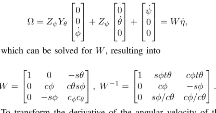
For simulations we want to express the dynamics of the quadcopter in the inertial frame. To transform the angular velocityΩof the body fixed frame to the angular velocityη˙ in the inertial frame,Ω =Wη˙ or η˙ =W−1_Ω_{, we use the same}

mapping of (yaw - pitch - roll). Assuming small changes, the

matrix will first have to be rotated before it can be transformed, requiring two transformations for the first angle, one for the second and none for the last, resulting in

Ω =ZψYθ

   0 0 ˙ φ  

+Zψ

   0 ˙ θ 0   +    ˙ ψ 0 0   =Wη,˙

which can be solved forW, resulting into

W =





1 0 −sθ

0 cφ cθsφ

0 −sφ cφcθ



, W−1=





1 sφtθ cφtθ

0 cφ −sφ

0 sφ/cθ cφ/cθ



.

To transform the derivative of the angular velocity of the body fixed frame to the inertial frame we require the derivative of the transformation.

¨

η= d

dt(W

−1_{Ω) =} d dt(W

−1_{)Ω +}_W−1_Ω_˙ ₍₁₁₎

where _dtd(W−1₎ _{is given by}

d dt(W

−1_{) =} 

 

0 φcφtθ˙ + ˙θ_csφ2_θ −φsφtθ˙ + ˙θ cφ c2_θ

0 −φsφ˙ −φcφ˙

0 φ˙cφ_cθ + ˙θsφtθ_cθ −φ˙sφ_cθ + ˙θcφtθ_cθ 

 

The simulation can then be solved by using equations, (6), (7) and (11), resulting in

¨

ξ=−gez+ 1

mRT−

1

mCξ˙ (12)

¨

η= d

dt(W

−1_{)Ω +}_W−1_I−1₍₋_Ω_×_IΩ₋_G₊_τ) ₍₁₃₎

where the equations (12) and (13) represent the UAV in the inertial frame with Ω =Wη˙.

B. Path planning

A path has to be calculated on which the UAV has to travel, which has to be done rather quickly because the UAV has to travel the moment a destination is known. Therefore the calculation is a trade-off between optimality and speed, as an optimal solution tends to take more time to calculate.

Several methods exist to create a path, [13] gives an overview of the methods available for path planning.

Our group system is solved using a graph approach, due to this we also employ a graph approach to generate the path. To find the path on a grid several methods can be used. The A* algorithm [14] or the Dijkstra’s algorithm [15] are well known algorithms for a graph approach; both ensure that the shortest path will result. In some cases the A* algorithm can be faster, because Dijkstra’s algorithm visits the closest vertex that it has not visited yet to see if it is the destination, while the A* algorithm allows heuristics and can prefer a direction. For this we employ the A* search algorithm which will generate a set of points that represent the path that will have to be taken by the UAV.

(12)

9 paths are calculated and, as is said for the event handling in Section I-A, the combination that is shortest is selected. In case several combinations of paths have the same length, the combination that is shortest and, if possible, has no overlapping paths that can cause collisions, is selected.

y

10 20 30 40 50 60 70 80 90

10 20 30 40 50 60 70 80

90 Starting point_{Target point}

A* path

Fig. 6. A* shortest path for a 100x100 grid.

C. Controller

A controller is required to control the quadcopter, in par-ticular we are interested in a controller that makes it possible to follow a path and stay in one position. The Crazyflie 2.0 has a built-in attitude control available. No internal software changes will be done to the quadcopter, therefore a controller using the available attitude PID control will have to be created. A quadcopter can be controlled by changing the thrust of the four propellers, as can be seen in equation (6), which also shows that in order to make the quadcopter move, the roll and pitch have to be controlled to cause a change in the rotational matrix, which then causes a change in the direction of the thrust and, assuming small angles, displacement to the direction it is leaning to.

The control inputs of the quadcopter are shown in equa-tion (8). By making sure that ω1 6= ω3, a pitch is achieved, the same goes for ω2 6=ω4 which will cause roll. A change in the yaw can be achieved by settingω1+ω36=ω2+ω4

If small angles are assumed for the roll and pitch, the setpoints of the roll and pitch can be linearized and be used as the desired velocity, meaning that the more the quadcopter leans towards a direction, the faster it will go into that direction, assuming that the altitude control responds faster and keeps the quadcopter levelled.

Movement through an area can be done in several ways; using just the destination as a set-point and apply PID po-sition control to go there is possible, but can easily lead to collisions or situations where the destination cannot be reached, additionally position control with waypoints cause the quadcopter to converge to each waypoint that it has to visit, thus slowing it down. Solutions to this are possible but not elegant, as is shown in Appendix C. Therefore we split

the type of control into Position controlto stay at a position and Path following control to follow a path. An overview of the complete controller is shown in Fig. 7.

Fig. 7. Control scheme of the system, the quadcopter has an inputω[1...4]

which is controlled by an attitude controller that controls based on the angle of the quadcopter. Depending on the selection of the position controller or the path following controller, a desired control action is generated, the resulting desired control action is then processed by the obstacle avoidance and send to the attitude controller.

1) Position control: For the position control a PID con-troller is used; it is easy to implement and only needs to make sure that the quadcopter stays in one position. Because we assumed that for small angles the change of angles can be considered as setting a velocity, the position control becomes rather straightforward. The error will be the difference of the current position and the desired position and the output will be a velocity in the direction of the error. The output will have to be transformed to take in account the yaw of the quadcopter, thus

" v0

x v0

y #

=

cosφ −sinφ

sinφ cosφ

vx vy

. (14)

2) Path following: To follow the path we use a similar method as is described in [16] and [17]: we set a position error that we want to minimize normal to the line that goes from the previous waypoint to the next waypoint, and a desired velocity in the tangent direction of the path. This allows us to move through a set of waypoints without stopping or converging to each of them, which happens if position control is used for the waypoints. The definition of the path as described in [17] is used,P∈N×R3, a sequence ofN waypoints,xiand desired

velocity vi along the path segment Pi connecting waypoint i

toi+1, and the current positionx(t). The cross-trackecterror of this method can be defined as

ect= (xi−x(t))˜n+ (xi−x(t))˜b (15)

wheren˜ is the normal and˜bthe unit vector to the track. This way we can minimize the cross-track error and still move along it, because the position control does not take in account the tangent direction. No separate controller is required for tangent direction, setting the velocity in the tangent direction corresponds to sending a setpoint to the built-in controller directly. Transition to the next path segment occurs when the UAV iscerror distanced from the plane normal to the path at the end of the segment. The path following is schematically depicted in Fig. 8.

(13)

v

ect

cerror

Fig. 8. Graphical overview of the path following system.

the desired velocity is. That means that vmax would be a straight line andvmina 90 degree turn. To get the curvature for our waypoints we approximate it using a circumcircle, using 3 sequent waypoints to find a unique radius that can represent the curvature. A large radius would indicate an almost straight line, while a small radius would indicate a sharp turn.

The circumcircle of three points can be determined by solving the following determinant

det

x2₊_y2 _x _y ₁

x2

1+y21 x1 y1 1 x2

2+y22 x2 y2 1 x2

3+y23 x3 y3 1

= 0 (16)

where(x, y)is the set of points of the circumcircle and(xi, yi)

the i-th point. The determinant can be written in the form

(x−x0)2+ (y−y0)2 =r2_{, resulting in a radius}_r _{from the}

three points, as is shown in Appendix D.

The resulting radiusrwill result into∞when all the points are on a straight line, to make use of this the desired velocity is based on the inverse of the radius, making it zero, the following application is proposed

f(r) = (

(vmax−vmin)−c1

r if (vmax−vmin)− 1 r >0

0 if (vmax−vmin)−1_r ≤0

vdes(r) =f(r) +vmin,

wheref(r)is a function that scales the velocity based on the inverse radius, and makes sure thatvmax can be achieved and that possible results of (vmax−vmin)− 1_r are 0 for values lower then 0, this to ensure thatvminis achieved. The constant

c∈_Rcan be used to tune the function.

An example of the method is shown in Fig. 9, the z axis describes how many degrees are desired for the velocity in the tangent direction, degrees is used due to the linearization of the velocity for the roll/pitch of the quadcopter.

D. Collision avoidance

To ensure that no crashes occur an avoidance algorithm is proposed, that has to ensure that the UAVs are not able to hit each other. For this the following safety system is used:

The system works on the fact that when UAVs are near each other and have no velocity direction towards each other, that they will not crash. No movement towards other UAVs means that it is not possible to collide based on the movement direction. The avoidance strategy checks all UAVs in a radiusr

around each UAV,rshould be large enough for the UAV to be

1

0.5

x (m)

0 -0.5

-1 -1 -0.5 0

y (m)

0.5 4

1.5

1 2

0.5 2.5 3 3.5

1

Angle (degree)

Fig. 9. Example of the velocity profile generation method, with vmax =

0.065rad,vmin= 0.015rad andc= 0.15, of a Lissajous figure.

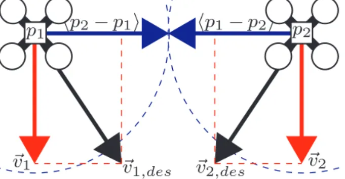
able to get to a standstill. For each surrounding UAV the veloc-ity vector is decomposed based on the direction vector between the UAV and each surrounding UAV, and saves the resulting tangent vector as the new desired velocity if the normal vector is positive; a negative normal vector would mean that the UAVs are moving away from each other. An example of this is shown in Fig. 10 and the algorithm is shown in Algorithm 1.

v

1

_v

v

2

1,des

v

2,des

p

1

−

p

2

p

2

−

p

1

p

1

p

2

Fig. 10. Representation of the avoidance system: The desired velocity is shown as~v#,des.~v# shows the new velocity, which is based on

the normal vector of the desired velocity decomposed into the unit vector that points towards the other UAV within the collision circle, which is shown with the dotted circle.

V. SIMULATIONS

Simulations are used to confirm the proposed architecture.

A. Hardware

(14)

Algorithm 1 Avoidance

Input: ~vN,des,pN,ψN,r Output: ~vN

1: foralln∈N do //~vn,desto the inertial frame

2: ~vn,inertial =Rot(−ψn)~vn,des

3: end for

4: foralln∈N do // Remove conflicting parts of~v

5: foralli∈N\ndo

6: if (||pi−pn||< r)then

7: pˆ= pi−pn

||pi−pn|| // Get the normal unit vector

8: ptanˆ =Rot(π₂)ˆp // Get the tangent unit vector 9: vnorm= ˆp0~vn,inertial // Decompose the velocity 10: vtan = ˆp0_tan~vn,inertial

11: ifvnorm>0 then

12: ~vn,inertial=vtan~ptan

13: end if

14: end if

15: end for

16: end for

17: foralln∈N do //~vn,inertialto the body-fixed frame

18: ~vn =Rot(ψn)~vn,inertial

19: end for

20: return ~vN

Gazebo [21] and MATLAB. ROS is a robotic aimed frame-work that allows, in combination with the simulator Gazebo, an easy transfer from simulation code to experimental code. MATLAB is used for the Group system and the MATLAB ROS I/O [22] package is used for the communication with ROS.

The simulation was split between 20-sim and Gazebo be-cause the initial design was done in 20-sim. The designed system was tested and then implemented in ROS, Gazebo was used to simulate a quadcopter to test that the ROS package was implemented correctly. For the collision avoidance a radius of 50 centimetres was used. A Lissajous figure is used to generate a path, this allows the velocity profile generation to be used effectively in the corners, to ensure that the quadcopter does not overshoot the path. The Lissajous figure also makes it possible to recreate the path easily, which ensures that the same path is used for all simulations and experiments. For the simulations in Gazebo a quadcopter implementation of [23] was used and for the velocity profile of the simulations the same parameters as Fig. 9 were used.

B. Results 20-sim

Two simulations are made, one is made with a quadcopter following a Lissajous figure, showing the effectiveness of the path following controller and velocity generation, and one with two identical quadcopters that follow a Lissajous figure, having starting positions opposite to each other moving the opposite directions, this to ensure that a collision occurs.

Fig. 11 shows the simulation result of a quadcopter follow-ing a Lissajous figure: The trajectory is closely followed except for the corners. Fig. 12 shows the cross-track error along the path: The error slightly exceeds six centimetres in the corners, a lower error can be achieved by changing the velocity profile.

y

(m)

x(m)

Fig. 11. Quadcopter following a Lissajous figure, starting atx = 0,

y= 1and moving clockwise. Simulated in 20-sim

y

(m)

Time (seconds)

Fig. 12. Error of the quadcopter following a Lissajous figure. Simulated in 20-sim.

Fig. 13 shows the simulation result of the quadcopter fol-lowing a trajectory. The trajectory is shown, two quadcopters, on opposite ends, are started at the same time and meet each other in the middle, at this point the obstacle avoidance takes control due to the quadcopters heading into a collision and ensures that the quadcopters do not collide.

The cross-track error is shown in Fig. 14. It can be seen that the error is closely followed, except for when the two UAVs are in collision. The saw like response is due to the approximation of the desired velocity, which consists out of 150 points of Fig. 9.

C. Results ROS

The system that was modelled in 20-sim is implemented in ROS. To test that the system does indeed show similar behaviour a simulation of it was made using Gazebo, for which a quadcopter implementation of [23] was used.

(15)

y

(m)

x(m)

Fig. 13. Path of the quadcopter following a Lissajous figure while avoiding another quadcopter, both quadcopters start atx= 0. Simulated in 20-sim.

y

(m)

Time (seconds)

Fig. 14. Error of the quadcopter following a Lissajous figure while avoiding another quadcopter. Simulated in 20-sim.

does show a slightly larger error around four seconds which corresponds to the first corner. This is due to the attitude controller that is different for the 20-sim model and Gazebo model. The UAV is having too much acceleration after it starts from no movement, causing it to overshoot.

The implementation of the avoidance using ROS is shown in Fig. 16. No collision occurs and the system shows the same behaviour as the 20-sim model with a similar cross-track error.

D. Results MATLAB

The implementation of the group system was realized using MATLAB and is shown in Fig. 17. There is no difference for the system for simulation application or experimental because it only uses the position data to generate paths. The desired position where an event appears is due to user action.

Fig. 17 shows an application of the system, all optimal distributions were calculated beforehand using the results of the optimal coverage problem. The background shows the

x (m)

-1 -0.5 0 0.5 1

y (m)

-1 -0.5 0 0.5 1 1.5

UAV Desired Path

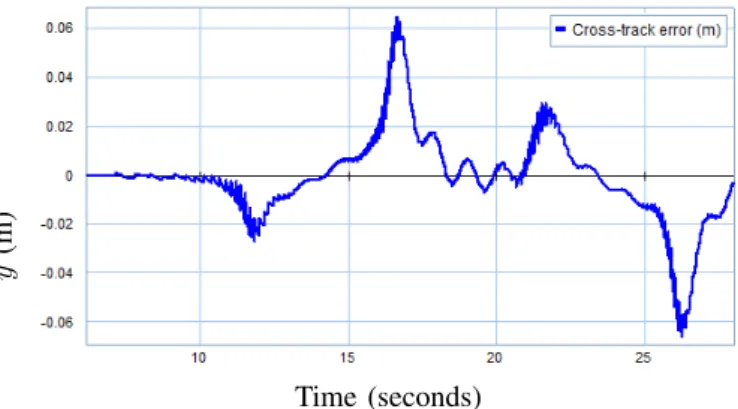
Time (seconds)10 20 30

Cross-track error (m)

-0.1 -0.08 -0.06 -0.04 -0.02 0 0.02 0.04 0.06 0.08

Fig. 15. Path following of a Lissajous figure, showing both the path and the cross-track error. Simulated in ROS/Gazebo

x (m)

-1 -0.5 0 0.5 1

y (m)

-1 -0.5 0 0.5 1

1.5 Desired path

UAV1 UAV2

Time (seconds)

4 6 8 10

-0.1 -0.05 0 0.05

0.1 UAV1

UAV2

Fig. 16. Path following of a Lissajous figure while avoiding another quadcopter, showing both the path and the cross-track error, both quadcopters start atx= 0. Simulated in ROS/Gazebo.

regions of each UAV. At Fig. 17(a) the system is enabled, from the current positions of the UAVs a path is generated towards the optimal placing of the UAVs according to the optimal coverage for 3 available UAVs and the desired positions are achieved in Fig. 17(b). In Fig. 17(c) two points in the area are selected, for which paths are generated for the two closest UAVs and the available UAV 3 is sent to the optimal coverage position, the centre. In Fig. 17(d) UAV 1 reaches the desired position, at which the system sends it back to the optimal coverage for 2 UAVS, which requires both available UAVs in the middle. When UAV 2 reaches its desired position in Fig. 17(e), 3 UAVs are available, for which the systems generates paths to move the UAVs, the final positioning is then achieved Fig. 17(f), which is similar to Fig. 17(b).

VI. EXPERIMENTS

For practical confirmation of the proposed architecture, experiments are performed based on the simulations.

A. Hardware

(16)

y

(m)

-3 -2 0 1 2 3

-3 -1 0 1 2 3

-1 -2

2

3

1

(a)

-3 -2 -1 0 1 2 3

1 2

3

(b)

-3 -2 -1 0 1 2 3

1 3 2

(c)

-3 -2 -1 0 1 2 3

1

3 2

(d)

-3 -2 -1 0 1 2 3 -3

-2 -1 0 1 2 3

1 3 2

(e)

-3 -2 -1 0 1 2 3 -3

-2 -1 0 1 2 3

1 3 2

(f)

x(m)

Path

#

UAV #

(g) Legend

Fig. 17. Example of the group system showing the UAVs and the paths they take.

Fig. 18. Overview of the experimental setup.

keep track of the quadcopter; it allows a 100 Hz position and attitude tracking. An overview of the setup is shown in Fig. 18. For the actual experiment the Crazyflie 2.0 was used, fitted with retroreflective markers as is shown in Fig. 19, carbon tubes were used to keep additional weight as low as possible due to the maximum recommended payload of 15g.

Fig. 19. Photograph of the Crazyflie 2.0 that are used.

B. Results

(17)

x (m)

-1 -0.5 0 0.5 1

y (m)

-1 -0.5 0 0.5 1 1.5

UAV Desired Path

Time (seconds)

0 5 10 15 20

-0.15 -0.1 -0.05 0 0.05 0.1 0.15 0.2 0.25

Fig. 20. Path following of a Lissajous figure, showing both the path and the cross-track error.

To get a better understanding of the large error in the system the position control error is also looked at, which is shown in Fig. 21. For the control thex-direction andy-direction used the same control settings. It can be seen that for thex-direction the error is within a band of 15 centimetres and shows a slight offset to the negative side, the y direction has a larger error band of 25 centimetres, and shows less control actions. The markers were attached in they-direction, which explains the different results. A better result might be gained if the attitude control is tuned to take in account the additional mass due to the markers, which affects the roll.

Time (seconds)

0 5 10 15 20

Error y (m)

-0.1 -0.05 0 0.05 0.1 0.15

Time (seconds)

0 5 10 15 20

Error x (m)

-0.15 -0.1 -0.05 0 0.05 0.1

Fig. 21. Error of the position control for thex-direction andy-direction.

VII. CONCLUSION

A working framework is proposed which allows the han-dling of events based on the minimization of costs over an area. The framework is designed and simulated, a practical implementation was tried but showed a large error, due to which the collision avoidance was not tested in practice.

For the optimal coverage problem that takes in account that events can require multiple UAVs, a control function is created which allows the calculation of optimal positions in an area based on density functions. The result of this allows the deployment of a group of UAVs on positions that are

calculated such that events can be serviced as optimal as possible.

The simulations of the UAV in both ROS/Gazebo and 20-sim achieved a low error while being able to follow a path using the generated velocity profile that is based on the angle the path makes, while the proposed collision avoidance ensured that no collisions occurred.

VIII. RECOMMENDATIONS

Several recommendations can be made for the framework. The event handling is currently managed on a come, first-served basis, which works by taking the closest UAV for the event. A better solution is to take in account that UAVs might be able to manage multiple events sequential and optimize for this.

A velocity controller might be able to improve the results of the set-up. Position control does not take in account the velocity, so while the desired position is achieved, it will overshoot due to the UAV still having a velocity.

It is not possible to compensate for the markers with just the current path following and position control, this requires tuning of the attitude control because it is a body-fixed problem.

The proposed collision avoidance is straightforward and does not allow for applications where multiple UAVs collide, when two UAVs are in a collision course the avoidance will stop the collision, but for a straight, head on collision, it means that both UAVs will stop and hover while not being able to continue. This is not desirable for a situation where events have to be serviced.

(18)

APPENDIXA ALGORITHM GROUP SYSTEM

The algorithm consists out of two parts, Algorithm 2 shows the part that calculates the Voronoi distribution based on a position, as is done in [10], Algorithm 3 uses the results of Algorithm 2 to calculate a new position that can be used for the next iteration, which takes in account the optimization for multiple UAVs that is proposed in Section III.

Algorithm 2 {τ, I}=Tessellation.Computation G,{pk},{Rk},φ, η¯

Input: graphG(with vertex setV(G), edge setE(G)⊆V(G)×V(G), and cost functionC(G) :E(G)→R+).

UAV locationspk ∈V(G), k= 1,2,· · · , N. UAV weightRk∈_R+_{, k}_{= 1,}_2,_{· · ·}_{, N}_.

Discretized density function φ¯:V(G)→_R. The metric tensor η:C →_RD×D_.

Output: The tessellation mapτ:V(G)→ {1,2,· · · , N}

The control integral I∈RD×D

1: Initiate g: Setg(v) :=∞ ∀v∈V(G) // Shortest distances

2: Initiate ρ: Setρ(v) :=∞ ∀v∈V(G) // Power distances

3: Initiate τ: Set τ(v) :=−1∀v∈V(G) // Tessellation

4: Initiate v: Setv(v) :=∅ ∀v∈V(G) // Pointer to robot neighbor.v:V(G)→V(G)

5: for each k∈ {1,2,· · ·, N} do

6: Set g(pk) = 0

7: Set ρ(pk) =−R2

k

8: Set τ(pk) =k

9: Set Ik = 0

10: for eachq∈NG(pk)do // For each neighbor ofpk

11: Set v(q) =q

12: end for

13: end for

14: Set Q:=V(G) // Set of un-expanded nodes

15: while Q6=∅ do

16: q:=argmin_q0_∈_Qρ(q0)

17: if (g(q) ==∞)then

18: break

19: end if

20: Set Q=Q−q // Remove q from Q

21: Set l:=τ(q)

22: Set s:=v(q)

23: if s! =∅then // Equivalently,q /∈ {pk}k=1,2,···,N

24: Set z= P(s)−P(pl)

||P(s)−P(pl)||2 // Unit tangent vector

25: M =η(P(pl)) // Metric tensor atplas a matrix

26: I(q) =g(q)×√M z

zT_{M z} ×φ¯(q)×

√ detM

27: end if

28: for eachw∈NG(q)do // For each neighbor ofq

29: Set g0 _:=_{g(q) +}_C_{(G)(q, w)}

30: Set ρ0 _:=_PowerDist_(g0_{, Rl)} 31: if ρ0 _{< ρ(w)}_then

32: Setg(w) =g0

33: Setρ(w) =ρ0

34: Setτ(w) =l

35: if s6=∅ then // Equivalently,q /∈ {pk}k=1,2,···,N

36: Set v(w) = s

37: end if

38: end if

39: end for

40: end while

(19)

The algorithm shown in Algorithm 2 is roughly the same as the algorithm that is proposed in [10], the main change is that the calculation of the position for the next iteration is removed and that instead the control integral is used as output. Algorithm 3 uses this control integral by calculating all control integrals for the UAVs of eachmrequired UAVs to be serviced, each mrequired UAVs consists out of a combination of possible UAVs that can be used for this requirement. By calculating the integral for each regions we can combine the control integrals of the tessellations and receive a global control integral, which takes in account all the combinations such that the UAVs are steered in the direction that has the most effect on the global cost.

Algorithm 3 {p0

k} = Position.Computation G,{pk},{Rk},φm, η¯

Input: graphG(with vertex setV(G), edge setE(G)⊆V(G)×V(G), and cost functionC(G) :E(G)→R+).

UAV locationspk ∈V(G), k= 1,2,· · · , N. UAV weightRk∈R+, k= 1,2,· · ·, N.

Discretized density function φm¯ :V(G)→R∀m∈ {1,2,· · · , M}.

The metric tensor η:C →RD×D. Output: The next position of each UAV, p0

k ∈NG(pk), k= 1,2,· · ·, N //p0kis a neighbour ofpk

1: {τ1, I0}=Tessellation.Computation G, K,{Rk},φm, η¯

// Calculate the initial Voronoi tessellations 2: for each i∈ {1,· · ·, N} do

3: QT1

i = find(τ1==i) // Get the initial area per UAV

4: Ii=sum(I0(QT1

i)) // Calculate the control action of UAVi

5: end for

6: c(1) =N // Set the amount of entries inT1

i, the maximum value fori

7: for each m∈ {2,· · ·, M}do

8: l= 0 // Set the initial amount of entries

9: for eachi∈ {1,· · · , c(m−1)}do// For each region of the previousm−1distribution we want to calculate the sub regions to create themdistribution

10: K={1,2,· · ·, N}

11: q=random(Q_Tm−1

i )

// A point in the region such that we can find the UAVs of the parent regions, random because any point is in the same parent region 12: for eachj ∈ {1,· · · , m−1} do

13: K=K\τTj(q) // Get the UAV on which the parent directoryjis based on and remove it from the set 14: end for

15: {τ0, I0}=Tessellation.Computation G, K,{Rk},φm, η¯

// Calculate the tessellation of the UAVs that could be them-th closest 16: for eachk∈ {1,2,· · ·, length(K)} do // Loop through each UAV and calculate the sub region it takes from the parent region 17: l=l+ 1

18: QTm

l = find(τ

0₌₌_k)_∩_Q

Tm−1

i

// Get the new sub-region 19: τTm(QTm

l ) =Kk // Keep a map which UAV takes which area

20: IK_k=IKk+sum(I

0_(QT_m

l )) // Add to the control action of UAVKk

21: end for

22: end for

23: c(m) =l

24: end for

25: for each k∈ {1,2,· · ·, N} do

26: Set p0

k :=argmaxu∈NG(pk)=

P(u)−P(pk)

||P(u)−P(pk)||2Ik

27: end for

(20)

APPENDIXB

GENERALIZATIONMETRICMANIFOLD

The proposed theory can also be generalized for any N-dimensional manifold that is equipped with a metric tensor. We can use the same methodology as is used in Section III and define a cost function based on a distance functiond(q, pi).

J(p, W) =

n X i=1 M X m=1 Z Wm i

fi(d(q, pi))φm(q) dq. (17)

We have to redefine our Zm

i regions to allow for a generic

distance function, thus let Zm

i = {q ∈ Ω : ∃H ⊂

{1. . . n}such that|H| =m−1, i6∈ H andfh(d(q, ph))≤ fi(d(q, pi))≤f`(d(q, p`))for allh∈H, ` /∈H, `6=i},

By definition Z minimizes J(p, W) as a function of W for fixedp, so we have

Jexp(p) =J(p, Z) = min

W J(p, W)

for everyp /∈C,whereC={p∈Ωn : ∃i, js.t.pi=pj}.

A. Gradient descent optimization

As in Section III-B we follow the gradient of the dynamics of the cost function to minimize it usingfi(x) =x2_.

∂J(P)

∂pk = ∂ ∂pk M X m=1 n X i=1 Z Zm i

d(q, pi)2φm(q) dq (18a)

= M X m=1 n X i=1 Z Zm i ∂

∂pkd(q, pi)

2_φm_{(q) dq} _(18b)

= 2 M X m=1 n X i=1 Z Zm i

d(q, pi) ∂

∂pkd(q, pi)φm(q) dq

(18c) = 2 M X m=1 Z Zm k

d(q, pk) ∂

∂pkd(q, pk)φm(q) dq (18d)

where for step (18a) to (18b) it is allowed to take the derivative under the integral according to [4, Proposition 2] and for step (18c) to (18d) the summation is removed because

∂

∂pkd(q, pi) = 0, ∀k6=i.

Equation 3 then becomes

˙

pi =−2κ M X m=1 Z Zm k

d(q, pk) ∂

∂pkd(q, pk)φm(q) dq (19)

which corresponds to steering each UAV towards a weighted “centre of mass” of its own responsibility region∪mZm

i . We

can then take

∂

∂pid(q, pi) =

P

jηij(pi)zqpj i

q P

m P

nηmn(pi)zqpmiz

n qpi

[3] (20)

where ηij(pk) is the metric tensor at point pk and zi qpk is

the ith component of the tangent vector atpk to the geodesic connectingqtopk. Since the objective function

dJ(p(t))

dt =

n X

i=1

∂J(p(t))

∂pi pi˙ =−κ

n X

i=1

_∂J_(p(t))

∂pi 2

is the same as in Section III-B we can use Proposition 1, thus the gradient dynamics converges to either the critical points of the cost or to configurations with coincident posi-tions.

APPENDIXC PATHFOLLOWING

A path following controller is required to ensure that the UAV is following the path, the path already avoids the obstacles so the path should be followed as good as possible. For any simulations in this appendix we consider the behaviour of the UAV as a point mass, F =m×a, with a mass of 1 kg andFmaxof 100 N. The path that we consider is a Lissajous curve, which is easy to generate and requires some action to follow it properly, all simulations are for 10 seconds.

A. Radius

Following a path can be done in several ways, a rather straightforward one is use a radius around the UAV, the waypoint that is the farthest away inside the radius is selected and is then used as a setpoint, as is shown in Fig. 22.

Fig. 22. Path following using a radius around the UAV and selecting the farthest away waypoint inside the circle schematically depicted.

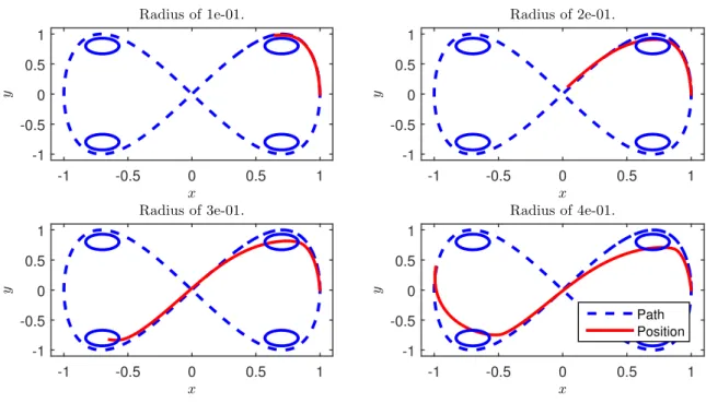
Fig. 23 shows the result of the simulation using a Lissajous curve as path around four obstacles, a simulation is shown for different radii. It can be seen that for small radii the simulation time is not enough but the path is followed, while for large radii more distance is travelled but the mass cuts-off corners, which causes it to collide with obstacles.

B. Error radius

A different approach to the radius following is to put a minimum radius on the error, this ensures that a minimum error has to be achieved before the next setpoint can be chosen. The results of this are shown in Fig. 24.

Fig. 24 shows the result of the simulation for different radii on the error. The radius that is used is the radius that the error has to be in before it can go to the next waypoint. It can be seen that for a large radius, the mass cuts off corners as was the same with the previous method. On the other side for low radii the system slows down because it first has to get closer to the setpoint before it can go to the next one.

(21)

x

-1 -0.5 0 0.5 1

y

-1 -0.5 0 0.5 1

Radius of 1e-01.

x

-1 -0.5 0 0.5 1

y

-1 -0.5 0 0.5 1

Radius of 2e-01.

x

-1 -0.5 0 0.5 1

y

-1 -0.5 0 0.5 1

Radius of 3e-01.

x

-1 -0.5 0 0.5 1

y

-1 -0.5 0 0.5 1

Radius of 4e-01.

Path

Position

Fig. 23. Path following with obstacles, select waypoint based on furthest waypoint in the radius.

x

-1 -0.5 0 0.5 1

y

-1 -0.5 0 0.5 1

Radius of 1e-01.

x

-1 -0.5 0 0.5 1

y

-1 -0.5 0 0.5 1

Radius of 2e-01.

x

-1 -0.5 0 0.5 1

y

-1 -0.5 0 0.5 1

Radius of 3e-01.

x

-1 -0.5 0 0.5 1

y

-1 -0.5 0 0.5 1

Radius of 4e-01.

Path Position

(22)

is greater than the set radius, while for the second simulation it is slightly larger in general. While for a straight trajectory the radius does not matter (except for the final point), it does matter for trajectories with curves, it is expected that for sharp curves a small radius is required to ensure that there are no corners cut-off.

The methods mentioned are usable but will require that the obstacle is not within the radius, thus the path always has to be around an obstacle at a distance at least equal to the radius. This indicated that a method has to be found which takes this in account and compensates for it, in case of the method that was used for the simulations this would mean that the radii have to be variable and change depending on the trajectory/change in direction.

While it is probably possible to come up with a method that changes the radius based on the trajectory and/or current state of the mass, a more simple method that takes in account the obstacle can be used.

Fig. 25. Path following line of sight schematically depicted.

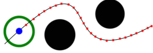
C. Line of sight

Fig. 25 shows an example of this method, by selecting the waypoint that is in the line of sight (LOS) of the mass, we ensure that the obstacle is not crossed, we can do this because we know the obstacles on which the path is based on.

x

-1 -0.8 -0.6 -0.4 -0.2 0 0.2 0.4 0.6 0.8 1

y

-1 -0.8 -0.6 -0.4 -0.2 0 0.2 0.4 0.6 0.8 1

Path Position

Fig. 26. Path following with obstacles using line of sight.

Fig. 26 shows result of using LOS, it is quite better than the previous two methods, half the trajectory is finished and no obstacles are crossed, this situation was not possible previously. The downside of this method is that the path is not followed, this is no problem in our case because it is shorter and faster, thus more optimal.

The problem with path following is that on a straight line we can go as fast as possible, while on a curved line we have to

slow down to ensure that we do not overshoot. The previous method is a simplification of this, when a path is curved it goes around an object, thus by selecting a waypoint that is seen we automatically compensate for the curve because we have to slow down because we do not see the next point yet. The downside of this method is that we cannot control the speed of the UAV because it fully depends on the waypoint that is in sight.

D. Curvature based path following

Vector to next point

Curvature

Adjusted vector

Fig. 27. Vector based path following schematically depicted.

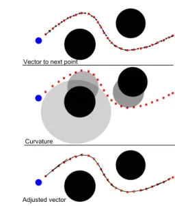
To get a method that compensates for the curvature we opt to change the waypoints of the path based on the curvature, as shown in Fig. 27. A good way to get the curvature is to estimate a circle/sphere through 3/4 points (depending on the dimension). This circle/sphere will have a radius, which we can use to change the waypoints. We move the waypoint in the direction of the path, thus the vector pointing to the next waypoint is lengthened based on the radius of the sphere/circle that goes through the points.

For the simulation the length of the vector was increased by a factor that was based on the curvature, the curvature 1_r of the circle that was intersection the waypoint and the next and previous waypoint was mapped, resulting in a value between 0 and 1. This radius was then used to calculate the factor which lengthens the vector pointing to the next waypoint, thus our set point. We usedc=k(1−1

r), instead of using r the inverse

was used, using r would result in an infinite radius when there is no curvature, this curvature 1_r is then subtracted from 1 to get a scaling where a small curve results in 0 and a straight line in 1.kis a constant which can be tweaked. The resulting factorcis then used to lengthen the vector pointing to the next waypoint.

Fig. 28 shows the result of using the curvature based path following, the result is quite better than the previous methods but requires some tweaking for it to work. in the simulation

(23)

x

-1 -0.8 -0.6 -0.4 -0.2 0 0.2 0.4 0.6 0.8 1

y -1 -0.8 -0.6 -0.4 -0.2 0 0.2 0.4 0.6 0.8 1 Path Position

Fig. 28. Vector adjusted path following with obstacles.

APPENDIXD

CIRCUMCIRCLE CALCULATION

There are 3 points in space that we want to connect using one circle, also known as a circumcircle, from which we want to know the radiusr∈_R,

P1= [x1, y1]∈_R2 P2= [x2, y2]∈R2 P3= [x3, y3]∈R2,

these 3 points can be connected trough one circle, for this the following constriction holds,

|P1−P0|=r2 (21)

|P2−P0|=r2 (22)

|P3−P0|=r2, (23)

whereP0 = [x0, y0]∈R2 is the centre point of the

circum-circle, the set of points P = [x, y] ∈R2 of the circumcircle

can then be described by|P−P0|=r2_.

A solution to these equations can be found by putting them into a matrix formAx= 0, and solving the determinant ofA

for det(A) = 0, as long as the kernel of Ais non-zero. The matrix form can be found by expanding the equations

|P−P0| −r2= (x−x0)2+ (y−y0)2−r2

=x2−2xx0+x20+y2−2yy0+y02−r2

=|P|2−2xx0−2yy0+|P0|2. (24)

Doing the same for equations (21), (22) and (23) results into

|P|2−2xx0−2yy0+|P0|2= 0 |P1|2₋_2x1x0₋_2y1y0₊_|_P0_|2_{= 0} |P2|2−2x2x0−2y2y0+|P0|2= 0 |P3|2−2x3x0−2y3y0+|P0|2= 0,

which can be written in the matrix formAx= 0 as



  

|P|2 ₋_2x ₋_2y ₁

|P1|2 ₋_2x1 ₋_2y1 ₁

|P2|2 ₋_2x2 ₋_2y2 ₁

|P3|2 ₋_2x3 ₋_2y3 ₁

        1 x0 y0 |P0|2

    =     0 0 0 0     , (25)

which has a non-zero kernel. By solving the det(A) = 0 we can gain an expression for the radius r of the circumcircle. For this we apply column operations to the matrix Ato get to the following expression

det 

  

|P|2 _x _y ₁

|P1|2 _x1 _y1 ₁

|P2|2 _x2 _y2 ₁

|P3|2 _x3 _y3 ₁



  

= 0. (26)

Solving the determinant leads to

D1|P|2+D2x+D3y+D4= 0 with (27)

D1=det





x1 y1 1

x2 y2 1

x3 y3 1



 D2=−det





|P1|2 _y1 ₁

|P2|2 _y2 ₁

|P3|2 y3 1





D3=det





|P1|2 _x1 ₁

|P2|2 _x2 ₁

|P3|2 _x3 ₁



 D4=−det





|P1|2 _x1 _y1

|P2|2 _x2 _y2

|P3|2 _x3 _y3



.

Equation (27) can then be rewritten as

D1(x+ D2

2D1)

2₊_D1(y₊ D3

2D1)

2₋ D22

4D1 −

D2 3

4D1 +D4= 0

D1(x+ D2

2D1)

2₊_D1_(y₊ D3

2D1)

2₌ D22

4D1+

D2 3

4D1 −D4

D1(x+ D2

2D1)

2₊_D1_(y₊ D3 2D1)

2₌ D22+D23−4D1D4 4D1

(x+ D2

2D1)

2_{+ (}_y₊ D3 2D1)

2₌ D22+D23−4D1D4 4D2

1

. (28)

Equation (28) corresponds to a circle of the form(x−x0)2+ (y−y0)2=r2_{, with the central point} _x0₌₋D2

2D1. y0= D3 2D1

and radiusr= √

D2

2+D23−4D1D4

2D1 , which is the circumcircle of

3 points.

APPENDIXE MANUAL

This appendix elaborates on how to use the software pack-age that was developed based on the proposed architecture. The package is available through the Robotics and Mecha-tronics group of the University of Twente.

A. Prerequisites

The software package is written for ROS, at the date of writing the current version of ROS is Indigo, which currently only supports Saucy (13.10) and Trusty (14.04) for Debian packages. The software was written based on ROS Indigo.

The following prerequisites are assumed for this manual: 1) Ubuntu 14.04 or any derivative based on this (Xubuntu

14.04, Lubuntu 14.04, etc).

(24)

3) Matlab R2013b with MATLAB I/O package.

4) Crazyflie client (https://github.com/bitcraze/crazyflie-clients-python)

5) Clean catkin workspace.

6) Knowledge on how to use Optitrack.

B. Installation

The package requires three main external packages, hector quadrotor (http://wiki.ros.org/hector quadrotor) for the simulation of a quadcopter, crazyflie ros (http://wiki.ros.org/crazyflie) to connect to the crazyflie and mocap optitrack (http://wiki.ros.org/mocap optitrack) to read the Optitrack data in ROS. The package that is available works with the currently available versions of these packages, using the latest version of the packages might be interesting but can be incompatible, therefore the current version will be included in the package.

After unpacking the package in the catkin workspace ex-ecute the following command in the workspace to solve dependencies.

$ r o s d e p i n s t a l l −−from−p a t h s r c

−−i g n o r e−s r c

This will install all required packages, the installation will request confirmation of installing the packages several times. The catkin workspace can now be compiled using the com-mand.

$ c a t k i n m a k e

It might be required to execute the command several times before the package compiles completely.

C. Usage

The interface can be started by executing the command

$ r o s r u n r a m c r a z y i n t e r f a c e . py

An example on what the interface looks like is shown in Fig. 29, the toggle buttonSimulationallows for the option to start the system with or without simulation, depending on the selection the ROS publisher and subscriber topics are changed. The Add Drone button adds drones, the response of this is shown in Fig. 30.

The table shows several columns, the Address shows the radio address that is used to connect to the drone, currently it is not possible to use more than one drone per radio. The first number shown is the radio ID, the second the drone ID and the third the bandwidth. The current configuration starts with the first drone at zero and increments by 60 for each additional drone, this can be changed in the interface code. ThePrefixcolumn is used by ROS to distinguish each drone. The Trackable ID is used by Optitrack, this ID will have to be set in the Optitrack interface to send the data to ROS. The Activecolumn shows if a controller is active.

If the simulation is selected Gazebo will have to be started manually, this can be done by executing the following com-mand.

Fig. 29. Example of the interface after start up.

Fig. 30. Example of the interface with 3 drones added.

$ r o s l a u n c h r a m c r a z y

q u a d r o t o r e m p t y w o r l d . l a u n c h

Double clicking on a row will activate the controller for that drone, a new window will appear. The interface that will appear is shown in Fig. 31. In this interface the following things can be done. The buttons on top will allow for the drone to take-off, land, or get the current setpoint of the drone. In case a simulation is used, the Spawn Simulation toggle will allow the deployment of the drone in the simulation, as shown in Fig. 32, when no simulation is used theToggle Radiotoggle can be used to enable the transmission to the drone using the radio dongle. In all cases thePublish Setpointtoggle will have to be enabled before any data is send. Data can be saved using the rosbag package, the Save Data toggle enables this and saves it to the standard ∼/.ros/ folder. A Lissajous path test will be executed if the Lissajous test toggle is enabled.

The interface allows the ability to set a position setpoint using the sliders, the offset thrust can also be set. The PID values for the Position control and Path Following control can be set, and send to the controller by pressing the Set gains button. An offset is available to compensate for a static error, the Get Current button allows the current I-action to be read and send to the interface, this way the offset can be determined using the I-action of the PID controller.

It is not possible to change the collision radius in the interface, nor the settings for the velocity profile generation based on the curvature, these settings will have to be changed in the code directly.

(25)

Fig. 31. Example of the interface after start up.

Fig. 32. Example of the interface with 3 drones added.

Fig. 33. Visualization of the system using RViz, the path is shown, the orientation of the UAV and the velocity vector.

Fig. 34. MATLAB group system.

REFERENCES

[1] Sherpa introduction. [Online]. Available: “http://www.sherpa-project.eu/ [2] J. Cortes, S. Martinez, and F. Bullo, “Spatially-distributed coverage op-timization and control with limited-range interactions,”ESAIM: Control, Optimisation and Calculus of Variations, vol. 11, no. 04, pp. 691–719, 2005.

[3] S. Bhattacharya, R. Ghrist, and V. Kumar, “Multi-robot coverage and exploration in non-Euclidean metric spaces,” inAlgorithmic Foundations of Robotics X. Springer, 2013, pp. 245–262.

[4] L. Pimenta, V. Kumar, R. Mesquita, and G. Pereira, “Sensing and cov-erage for a network of heterogeneous robots,” in47th IEEE Conference on Decision and Control, Canc´un, Mexico, Dec 2008, pp. 3947–3952. [5] P. Surynek, “An optimization variant of multi-robot path planning is

intractable.” inAAAI, 2010.

[6] J. Van den Berg, M. Lin, and D. Manocha, “Reciprocal velocity obstacles for real-time multi-agent navigation,” inRobotics and Automation, 2008. ICRA 2008. IEEE International Conference on. IEEE, 2008, pp. 1928– 1935.

[7] J. Van Den Berg, S. J. Guy, M. Lin, and D. Manocha, “Reciprocal n-body collision avoidance,” inRobotics research. Springer, 2011, pp. 3–19.

[8] D. M. Stipanovi´c, P. F. Hokayem, M. W. Spong, and D. D. ˇSiljak, “Cooperative avoidance control for multiagent systems,” Journal of Dynamic Systems, Measurement, and Control, vol. 129, no. 5, pp. 699– 707, 2007.

[9] F. Bullo, J. Cort´es, and S. Mart´ınez, Distributed Control of Robotic Networks, ser. Applied Mathematics Series. Princeton University Press, 2009.

[10] S. Bhattacharya, R. Ghrist, and V. Kumar, “Relationship between gradient of distance functions and tangents to geodesics,” Technical report, University of Pennsylvania, http://subhrajit.net/wiki/index.php, Tech. Rep.

[11] Bitcraze: The Crazyflie 2.0 product page. [Online]. Available: “https://www.bitcraze.io/crazyflie-2/

[12] T. Hamel, R. Mahony, R. Lozano, and J. Ostrowski, “Dynamic modelling and configuration stabilization for an x4-flyer.”a a, vol. 1, no. 2, p. 3, 2002.

[13] M. Elbanhawi and M. Simic, “Sampling-based robot motion planning: A review,”Access, IEEE, vol. 2, pp. 56–77, 2014.

[14] P. E. Hart, N. J. Nilsson, and B. Raphael, “A formal basis for the heuristic determination of minimum cost paths,”Systems Science and Cybernetics, IEEE Transactions on, vol. 4, no. 2, pp. 100–107, 1968. [15] M. Sniedovich, “Dijkstra’s algorithm revisited: the dynamic

program-ming connexion,”Control and cybernetics, vol. 35, no. 3, p. 599, 2006. [16] N. Michael, D. Mellinger, Q. Lindsey, and V. Kumar, “The GRASP multiple micro-UAV testbed,” IEEE Robotics Automation Magazine, vol. 17, no. 3, pp. 56–65, 2010.

[17] G. M. Hoffmann, S. L. Wasl, and C. J. Tomlin, “Quadrotor helicopter trajectory tracking control,” inAIAA Guidance, Navigation, and Control Conference, 2008.

[18] W. Hanna, “Modelling and control of an unmanned aerial vehicle,” Ph.D. dissertation, Charles Darwin University, 2014.

[19] 20-sim,version 4.5. Enschede, The Netherlands: Controllab Products B.V., 2015.

[20] ROS: An open-source robot operating system. [Online]. Available: “http://www.ros.org/

[21] Gazebo: Robot simulation made easy. [Online]. Available: “http://gazebosim.org/

[22] Matlab ROS I/O, A Downloadable MATLAB Add-On. [Online]. Available: “http://www.mathworks.com/ros

[23] J. Meyer, A. Sendobry, S. Kohlbrecher, U. Klingauf, and O. von Stryk, “Comprehensive simulation of quadrotor uavs using ros and gazebo,” in3rd Int. Conf. on Simulation, Modeling and Programming for Autonomous Robots (SIMPAR), 2012, p. to appear.