University of Warwick institutional repository: http://go.warwick.ac.uk/wrap
This paper is made available online in accordance with
publisher policies. Please scroll down to view the document
itself. Please refer to the repository record for this item and our
policy information available from the repository home page for
further information.
To see the final version of this paper please visit the publisher’s website.
Access to the published version may require a subscription.
Author(s): Rui Wang, Bo Wang, Guo-Ping Liu, Wei Wang, and David
Rees
Article Title: H∞ Controller Design for Networked Predictive Control
Systems Based on the Average Dwell-Time Approach
Year of publication: 2010
Link to published article:
http://dx.doi.org/ 10.1109/TCSII.2010.2043386
H
∞
Controller Design for Networked Predictive
Control Systems Based on the Average
Dwell-Time Approach
Rui Wang, Bo Wang, Guo-Ping Liu, Wei Wang, and David Rees
Abstract—This brief focuses on the problem of H∞ control for a class of networked control systems with time-varying delay in both forward and backward channels. Based on the aver-age dwell-time method, a novel delay-compensation strategy is proposed by appropriately assigning the subsystem or designing the switching signals. Combined with this strategy, an improved predictive controller design approach in which the controller gain varies with the delay is presented to guarantee that the closed-loop system is exponentially stable with an H∞-norm bound for a class of switching signal in terms of nonlinear matrix inequalities. Furthermore, an iterative algorithm is presented to solve these nonlinear matrix inequalities to obtain a suboptimal minimum disturbance attenuation level. A numerical example illustrates the effectiveness of the proposed method.
Index Terms—Average dwell-time method, H∞ control, net-worked control systems (NCSs), predictive control, switched system.
I. INTRODUCTION
N
ETWORKED control systems (NCSs) is a research area that has emerged in recent years [1]–[8]. A challenging aspect of networked control is that we need to compensate for the negative effects of the network constraints to retain the stability and performance of the system. For this purpose, one technique that has recently been proposed for NCSs is the networked predictive control (NPC) approach, which has been shown to be an effective approach to address this problem [9]– [11]. The main idea is that a sequence of future control predic-tions is generated at the controller node and transmitted to the actuator node, and then, at the actuator, an algorithm is used to choose the appropriate element from the received control prediction sequence as the actual control input according toManuscript received July 7, 2009; revised November 9, 2009 and January 11, 2010. Current version published April 21, 2010. This work was supported by China Postdoctoral Science Special Foundation under Grant 200902539. The work of G.-P. Liu was supported in part by the National Natural Science Foundation of China under Grant 60934006. This paper was recommended by Associate Editor M. Storace.
R. Wang is with the Research Center of Information and Control, Dalian University of Technology, Dalian 116024, China, and also with the Faculty of Advanced Technology, University of Glamorgan, Pontypridd CF37 1DL, U.K. (e-mail: [email protected]).
B. Wang is with the School of Engineering, University of Warwick, Coventry CV4 7AL, U.K.
G.-P. Liu is with the Faculty of Advanced Technology, University of Glamorgan, Pontypridd CF37 1DL, U.K., and also with the CTGT Center, Harbin Institute of Technology, Harbin 150001, China.
W. Wang is with the Research Center of Information and Control, Dalian University of Technology, Dalian 116024, China.
D. Rees is with the Faculty of Advanced Technology, University of Glamorgan, Pontypridd CF37 1DL, U.K.
Digital Object Identifier 10.1109/TCSII.2010.2043386
the measured network delay. Thus, the effect of the network delay is compensated. The resulting closed-loop system is transformed to a switched system. However, there are three limitations on the work reported in the publications to date. First, system stability has to be subject to arbitrary switching of all subsystems due to the random network delay. Therefore, existing papers are all based on a condition that all subsystems have to possess a common Lyapunov function. This condition is strict because sometimes some values of the network delay are not admissible when considering the system stability of NPC systems. Second, a fixed controller gain is used so that this re-sults in a significant conservative design because the controller gain does not reflect the range of possible delays in the network. Third, the design of the controller gain was not considered.
In this brief, to overcome the first limitation, a novel delay-compensation strategy for NPC systems is proposed by appro-priately assigning the subsystem or designing the switching signal. This strategy works, even if there exist unstable sub-systems, because they can be omitted in the assigning process. As for the remaining stable subsystems, it is not necessary to have a common Lyapunov function, but the overall system still may be stable under some suitable switching signals. The average dwell-time method is an effective tool for finding such switching signals [12]–[15]. To overcome the second and third limitations, an improved predictive controller scheme is designed in which the controller gain varies with the delay. In contrast with some existing references, which are based on the fixed controller gain approach, these varying feedback controller gains can lead to less conservative results. Based on the average dwell-time technique and this improved predictive controller scheme, the corresponding closed-loop system is exponentially stable with an H∞-norm bound. Moreover, an iterative algorithm is presented to design the desired controllers with a suboptimal minimum disturbance attenuation level.
II. PRELIMINARIES ANDPROBLEMFORMULATION
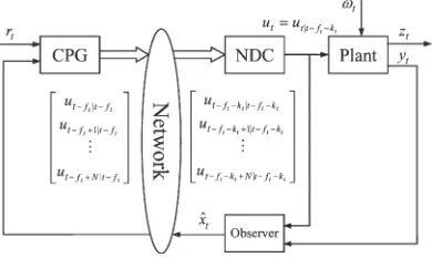
The NPC system structure is shown in Fig. 1. It includes two parts, namely, a control prediction generator (CPG) at the controller side and a network delay compensator (NDC) at the actuator side. The plant is modeled as follows:
xt+1=Axt+But+Ewt yt=Cxt zt=Dxt (1)
where xt∈Rn, ut∈Rm, and yt∈Rl denote the state
vec-tor, control input, and control output, respectively;zt∈Rp is
the output to be regulated; wt∈Rq is the disturbance input
belonging to L2(0,+∞); andA,B,C,D, andE are known
Fig. 1. NPC system structure.
constant matrices with appropriate dimensions.rt∈Rn is the
reference input. Without loss of generality, rt is assumed to
be zero throughout this brief. To measure the network delay, a time-stamp signal is transmitted together with the control predictions. In addition, the following assumptions are made.
Assumption 1: The upper bounds of the time-varying net-work delaysktin the forward channel and the feedback channel ftare not greater thanN1andN2, respectively, whereN1and
N2are positive integers, i.e.,kt∈{0,1, . . . , N1}andft∈{0,1, . . . , N2}, wheret= 0,1,2, . . .denotes the sampling instant.
Assumption 2: The numbers of consecutive data dropouts in the forward and feedback channels are less than L1 and L2,
respectively, both of which are positive integers. It is assumed that the upper bound number of consecutive data dropouts and network delay is equal toN =N1+N2+L1+L2.
III. PREDICTIVECONTROLSTRATEGY
A. Prediction of the Future Control Sequence
Since the system states are normally unavailable, the follow-ing state observer is designed:
ˆ
xt+1=Aˆxt+But+L(yt−Cxˆt) (2)
where xˆt∈Rn and ut∈Rm are the observed state and the
input of the observer, respectively, at time t, and L is the observer gain to be designed later. Note that the above observer is implemented at the plant side, as shown in Fig. 1. This is not a question for the modern “smart” actuator or sensor, which has the capacity to perform some not very complicated calculation, such as the calculation in the NDC and the observer here.
For the system without time delay, the controller is designed using the state feedback control strategy, i.e.,
ut=K0xˆt (3)
whereK0∈Rm×nis the control gain matrix to be determined.
When there are time-varying delays and data dropout in the feedback channel, the predictive controller from timet−ft+ 1totis generated by
ut−ft+i|t−ft=Kixˆt−ft
wherei= 1,2, . . . , ft,ft∈ {0,1, . . . , N2+L2}.
When time-varying delays and data dropout happen in the forward channel, the predictive controllers fromt+ 1tot+kt
is constructed as
ut+j|t−ft =Kft+jxˆt−ft
wherej= 1,2, . . . , kt,kt∈ {0,1, . . . , N1+L1}.
Thus, the state feedback controllers can be given as
ut=ut|t−kt−ft =Kft+ktxˆt−kt−ft
ft+kt∈N¯ ={0,1, . . . , N}. (4)
B. Assigning and Compensation of Network Delay
Assuming that the control sequence with network delaykt+ ftarrives at timet, then
Ut−kt−ft|t−kt−ft =
⎡ ⎢ ⎢ ⎢ ⎣
ut−kt−ft|t−kt−ft
ut−kt−ft+1|t−kt−ft
.. .
ut−kt−ft+N|t−kt−ft
⎤ ⎥ ⎥ ⎥ ⎦.
As aforementioned, if the element ut|t−kt−ft is chosen as the
control input, the impact of the network delay kt+ft on the
system performance is compensated.
However, from the perspective of system stability, some val-ues ofktandftare not permissible. Therefore, in this situation,
it is necessary to modify the network delay. Examining the ele-ments afterut|t−kt−ft in the sequenceUt−kt−ft|t−kt−ftenables
the control inputs at timet+i,i= 1,2, . . . , N−kt−ft,
re-spectively, to be used. This property enables us to assign the network delay we want. As for the elements beforeut|t−kt−ft,
they are just discarded.
Hence, all possible available control sequences (at least 1 and at mostN+ 1) are
Ut−N|t−N, Ut−(N−1)|t−(N−1), . . . , Ut|t
and the corresponding control input candidates are
ut|t−N, ut|t−(N−1), . . . , ut|t (5)
which result in the network delay
kt+ft=N, N−1, . . . ,0
respectively. The delay range is extended from 0∼N1+N2
to0∼N; thus, it is called extended network delay. It is worth noting that this delay assignment is not arbitrary because not all
N+ 1control input candidates are definitely available. Hence, it is called “partly assigning.”
Remark 1: Notice that all candidates keep the same form as (4); thus, any one of them can compensate the corresponding network delay. It can be seen that the compensation strategy (4) is a special case of the improved one (5).
IV. H∞CONTROLUSING APREDICTIVE
CONTROLLER FORNCSs
A. Stability andH∞Performance Analysis
According to the controller (4), the observer (2) can be written as
ˆ
xt+1= (A−LC)ˆxt+BKixˆt−i+LCxt, i∈N .¯ (6)
Thus, the closed-loop form of system (1) can be written as
xt+1=Axt+But+Ewt
The combination of (4), (6), and (7) gives the augmented switched system
¯
xt+1= ¯Aσ(t)x¯t+ ¯Ewt yt= ¯Cx¯t zt= ¯D¯xt (8)
whereσ(t)is called a switching signal, and
¯ xt=
xTt, xTt−1, . . . , xtT−i, xTt−i−1, . . . ,
xTt−N,xˆTt,xˆTt−1, . . . ,xˆTt−i, . . . ,xˆTt−N T ¯
E=
E 0(2N+1)n×q
¯
C= [C 0l×(2N+1)n] ¯
D= [D 0p×(2N+1)n] A¯i=
Π Ξi Φ Ωi
with
Π =
A 0n×N n IN n 0N n×n
Φ =
LC 0n×N n 0N n×n 0N n×N n
Ξi=
0n×in BKi 0n×(N−i)n 0(N+1)n×in 0(N+1)n×n 0(N+1)n×(N−i)n
Ωi=
A−LC 0n×(i−1)n BKi 0n×(N−i)n In I(i−1)n I(N−i)n 0N n×n
.
Lemma 1: Given γ0>0, if there exists a positive definite
matrixP such that
¯ AT
i PA¯i−P+ ¯DTD¯ A¯i T
PE¯
∗ E¯TPE¯−γ2
0I
<0 ∀i∈N¯
(9)
hold, then system (8) satisfies H∞ control under arbitrary switching.
Proof: Choose a common Lyapunov function as
Vt= ¯xtPTx¯t (10)
whereP is a positive definite matrix satisfying matrix inequal-ities (9). Along the trajectory of system (8), calculating the difference of Lyapunov function candidate (10), it is easy to
establish the above result.
Definition 2 [15]: Forα >0andγ0>0, system (8) is said
to satisfy weightedH∞control, if under a zero initial condition, it holds that
+∞
t=0
e−αtztTzt≤γ02 +∞
t=0
wTtwt. (11)
Assumption 3: Given γ0>0, we can design the
con-troller gainsKN1+N2, . . . , KN to make subsystems{A¯N1+N2,
¯
AN1+N2+1, . . . ,A¯N} have a common Lyapunov function so
thatH∞ control is satisfied for every subsystem. Namely, the matrix inequalities
¯
AT
i PA¯i−P+ ¯DTD¯ A¯TiPE¯
∗ E¯TPE¯−γ2
0I
<0,
∀i∈ {N1+N2, . . . , N}
have solutionP >0.
We can classify all subsystems of (8) into the following four categories:
Ψ1:{A¯N1+N2,A¯N1+N2+1, . . . ,A¯N};
Ψ2: Part of{A¯0,A¯1, . . . ,A¯N1+N2−1}that can be stabilized and
have a common Lyapunov function withΨ1;
Ψ3: Part of{A¯0,A¯1, . . . ,A¯N1+N2−1}that can be stabilized but
have no common Lyapunov function withΨ1;
Ψ4: Part of{A¯0,A¯1, . . . ,A¯N1+N2−1}that cannot be stabilized.
We use ψ1, ψ2, ψ3, and ψ4 to denote the subscript sets
to which the subsystems correspond to Ψ1,Ψ2,Ψ3 and Ψ4,
respectively.
We are now in the position to give the main result.
Theorem 1: Given α >0, γ0>0, if there exist matrices
¯
Pi>0such that
Π =
¯
AT
iP¯iA¯i−e−αP¯i+ ¯DTD¯ A¯TiP¯iE¯
∗ E¯TP¯iE¯−γ2
0I
>0
(12)
hold ∀i∈M =ψ1∪ψ2∪ψ3, then system (8) satisfies H∞
control for any switching signalσ(t) : [0,+∞)→M satisfy-ing the average dwell time
τa ≥τa∗= ln μ
α (13)
where
¯ Pi=
PN1+N2, i∈ψ1∪ψ2
Pi, i∈ψ3
andμ≥1satisfies
¯
Pi≤μP¯j ∀i, j∈M. (14)
Proof: Choose a Lyapunov function candidate as
Vt= ¯xTtP¯σ(t)x¯t (15)
where σ(t)∈M, P¯i are positive definite matrices satisfying
matrix inequalities (12).
Along the trajectory of system (8), for a Lyapunov function candidate (15), we have
Vt+1−e−αVt+ Γt= [ ¯xTt wTt ] Π
¯ xt wt
which then leads to the following based on (12):
Vt+1≤e−α(t+1)V0−
t
l=0
e−α(t−l)Γl
whereΓt=ztTzt−γ02ωtTωt.
For any time interval [0, t), let 0 =t0< t1<· · ·< tq = tNσ(t)denote the switching time instants ofσ(t). Thus
Vt≤e−α(t−tq)Vtq−
t−1
l=tq
e−α(t−l−1)Γl.
SinceVti≤μV
−
ti holds for every switching time instanttifrom
(14), we obtain by induction that
Vt≤e−αt+Nσ(0,t) lnμV0−
t−1
l=0
μNσ(l+1,t)e−α(t−l−1)Γl. (16)
Whenw= 0, we get from (16), under the conditionNσ(0, t)≤ (t/τa), that Vt≤e−(α−(lnμ/τa))tV0. Exponential stability
di-rectly follows from this inequality.
multiplyingμ−Nσ(0,t)on both sides of (16) yields
0≤ − t
l=1
μ−Nσ(0,l)e−α(t−l)Γl−1. (17)
Then, similar to the proof of Theorem 2 in [14], the result is easily obtained. The proof is completed. Remark 2: When μ= 1, P¯i= ¯Pj holds for any i, j∈M,
which means a common Lyapunov function exists for all sub-systems. For this case, from (17), the normalL2-gain directly
follows.
B. Design of anH∞Controller
In this section, we extend Theorem 1 to design the H∞
controller gainsKifor system (8).
Define matrices
B1=
B 0(2N+1)n×m
B2=
⎡
⎣0(N+1)Bn×m 0N n×m
⎤ ⎦
˜ I=
⎡
⎣0(N+1)Inn×n 0N n×n
⎤
⎦ C˜= [C 0p×N n −C 0p×N n]
I0= [ 0n×(N+1)n In 0n×N n] I1= [ 0n×(N+2)n In 0n×(N−1)n]
· · ·
Ii = [ 0n×(N+i+1)n In 0n×(N−i)n] ˜
Ai =
Π 0(N+1)n×(N+1)n 0(N+1)n×(N+1)n Π
whereΠis defined in Theorem 1. Then,A¯ican be written as
¯
Ai= ˜A+B1KiIi+ ˜ILC˜+B2KiIi. (18)
From (18), inequalities (12) are equivalent to the following matrix inequalities:
⎡ ⎣−e
−αP¯
i+ ¯DTD¯ 0 A¯Ti
∗ −γ2
0I E¯T
∗ ∗ −P¯−1
i
⎤
⎦<0, i∈M. (19)
In view of the above discussion, we can now obtain the following theorem.
Theorem 2: If there exist positive definite matricesP¯i>0, i∈M, such that∀i, j∈M matrix inequalities (19) hold, then system (8) with the controllers (4) is exponentially stable with theH∞-norm boundγ0.
Remark 3: The conditions for the H∞ controller analysis problem in Theorem 1 are difficult to solve becauseA¯icontain Ki andL. In Theorem 2, we separateKi and Lfrom A¯i to
obtain the controller gainKiandLby solving a set of LMIs.
It is noted that the conditions in Theorem 2 do not meet the LMI conditions because of the termsP¯iandP¯i−1. The problem
can be solved based on the method proposed in [16] By replacing the termP¯i−1in (19) byWi, we get
⎡ ⎣−e
−αP¯
i+ ¯DTD¯ 0 A¯Ti
∗ −γ2
0I E¯T
∗ ∗ −Wi
⎤
⎦<0, i∈M. (20)
Then, the minimization problem involving the LMI con-straints can be formulated as follows:
minimize trace( ¯PiWi)
subject to(20),
¯
Pi I I Wi
≥0, i∈M. (21)
C. Algorithm
The following iterative algorithm is presented, where (19) is a stopping criterion, since it is numerically very difficult in practice to obtain the optimal solution, and thus, only the suboptimal disturbance attenuation level γ0 can be obtained
within a specified number of iterations.
1) Choose a sufficiently large initialγ0such that there exists
a feasible solution to the LMI conditions in (20) and (21). 2) Find a feasible set ( ¯Pi, Wi, Ki, L (i∈M)) satisfying
LMIs in (20) and (21). Setk= 0.
3) Solve the following LMI problem for the variables
¯ Pi,Wi:
minimize trace( ¯PikWi+ ¯PiWik), i∈M.
subject to LMIs in(20)and(21).
4) If condition (19) is satisfied, then return to Step 2 after decreasing γ0 to some extent. If conditions (20) and
(21) are not satisfied within a specified number of iter-ations, then exit. Otherwise, setk=k+ 1,P¯ik+1= ¯Pi, Wik+1=Wi, and go to Step 3.
Remark 4: It is also noticed that the use of the cone-complementary algorithm has some disadvantages; for exam-ple, it requires more computing time and is memory consuming. Therefore, other alternative methods to solve the nonlinear matrix inequalities are worth exploring further, for instance, the method in [17].
V. SIMULATION
Consider NPC system (1) with the following system matrices:
A=
⎡
⎣0.48201.01 0.27100.1 −0.48800.24 0.0020 0.3681 0.7070
⎤ ⎦ B=
⎡ ⎣53 −52
5 4
⎤ ⎦
C=
1 2 3 4 3 1
D=
0.02 0 0.03 0.04 0.01 0.01
E= 0.01I
and the disturbance input, i.e.,
wt=
[ 1 1 1 ]T, 0< t≤2 0, t >2 .
This example is similar to the one in [11], where the distur-bance effect is not considered.
It is assumed that the upper bounds of the network delayskt
in the forward channel and the feedback channelftare all not
Fig. 2. Control inputs of system (1).
Fig. 3. Outputs of system (1).
Choosingα= 0.1andμ= 1.05, in all subsystems,A¯2,A¯3,
andA¯4 have common P; and A¯0 or A¯1 has no common P
withA¯2,A¯3, andA¯4and satisfy (19). Thus,σ(t) : [0,+∞)→
M ={0,1,2}. From (13), we getτa= 0.5≥τa∗ = 0.4879. By
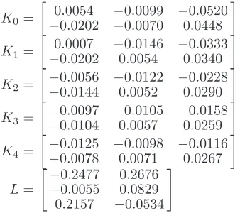
applying the algorithm to this example, the maximum itera-tion number is chosen to be 100. By applying the proposed algorithm in Section IV-C to this example, where the iteration number is chosen to be 100 and MATLAB/LMI Toolbox is used to solve the LMI problem, we obtain
K0=
0.0054 −0.0099 −0.0520
−0.0202 −0.0070 0.0448
K1=
0.0007 −0.0146 −0.0333
−0.0202 0.0054 0.0340
K2=
−0.0056 −0.0122 −0.0228
−0.0144 0.0052 0.0290
K3=
−0.0097 −0.0105 −0.0158
−0.0104 0.0057 0.0259
K4=
−0.0125 −0.0098 −0.0116
−0.0078 0.0071 0.0267
L=
−
0.2477 0.2676
−0.0055 0.0829 0.2157 −0.0534
and theH∞performance boundγ0= 0.02.
The control input and output trajectory of the system are shown in Figs. 2 and 3, respectively. It is easy to see that the system is stable and has acceptable performance.
Compared with our previous paper [11], the approach in this brief is a significant improvement for the following three reasons: First, the varying controller gains are easy to design,
whereas the fixed controller gain in [11] needs to be selected in advance. Second, the proposed approach can solve the four-step delay and higher delay problem, whereas employing the method in [11] can address only the three-step delay problem. Third, by using the method in this brief, it only takes 6 s to reach a stable response, whereas in [11], it takes approximately 100 s to reach a stable response.
VI. CONCLUSION
The problem ofH∞ control for a class of NPC systems has been studied in this brief. An improved compensation strategy based on the average dwell-time method was combined with a novel controller design approach to make the corresponding closed-loop system exponentially stable with the H∞ perfor-mance bound. In contrast with some existing methods, which are based on the fixed controller gain and common Lyapunov function, these varying feedback controller gains and multi-ple Lyapunov function matrices can lead to less conservative results.
REFERENCES
[1] G. C. Walsh and H. Ye, “Scheduling of networked control systems,”IEEE Control Syst. Mag., vol. 21, no. 1, pp. 57–65, Feb. 2001.
[2] A. V. Savkin, “Analysis and synthesis of networked control systems: Topological entropy, observability, robustness and optimal control,”
Automatica, vol. 42, no. 1, pp. 51–62, Jan. 2006.
[3] L. A. Montestruque and P. Antsaklis, “Stability of model-based networked control systems with time-varying transmission times,” IEEE Trans. Autom. Control, vol. 49, no. 9, pp. 1562–1572, Sep. 2004.
[4] Z. H. Mao, B. Jiang, and P. Shi, “Protocol and fault detection design for nonlinear networked control systems,”IEEE Trans. Circuits Syst. II, Exp. Briefs, vol. 56, no. 3, pp. 255–259, Mar. 2009.
[5] W. Zhang, M. S. Branicky, and S. M. Philipsm, “Stability of networked control systems,”IEEE Control Syst. Mag., vol. 21, no. 1, pp. 84–99, Feb. 2001.
[6] X. M. Tang and J. S. Yu, “Feedback scheduling of model-based networked control systems with flexible workload,”Int. J. Autom. Comput., vol. 5, no. 4, pp. 389–394, Oct. 2008.
[7] D. Yue, Q. L. Han, and P. Chen, “State feedback controller design of net-work control systems,”IEEE Trans. Circuits Syst. II, Exp. Briefs, vol. 51, no. 11, pp. 640–644, Nov. 2004.
[8] D. Yue, Q. L. Han, and J. Lam, “Network-based robustH∞control of sys-tems with uncertainty,”Automatica, vol. 41, no. 6, pp. 999–1007, Jun. 2005. [9] Y.-B. Zhao, G.-P. Liu, and D. Rees, “Networked predictive control sys-tems based on Hammerstein model,”IEEE Trans. Circuits Syst. II, Exp. Briefs, vol. 55, no. 5, pp. 469–473, May 2008.
[10] G.-P. Liu, Y. Xia, D. Rees, and W. Hu, “Design and stability criteria of networked predictive control systems with random network delay in the feedback channel,”IEEE Trans. Syst., Man, Cybern. C, Appl. Rev., vol. 37, no. 2, pp. 173–184, Mar. 2007.
[11] G.-P. Liu, Y. Xia, J. Chen, D. Rees, and W. Hu, “Networked predictive control of systems with random network delays in both forward and feedback channels,”IEEE Trans. Ind. Electron., vol. 54, no. 3, pp. 1282– 1297, Jun. 2007.
[12] J. P. Hespanha and A. S. Morse, “Stability of switched systems with average dwell-time,” inProc. 38th IEEE Conf. Decision Control, Dec. 1999, pp. 2655–2660.
[13] D. Liberzon, Switching in Systems and Control. Boston, MA: Birkhauser, 2003.
[14] X. M. Sun, J. Zhao, and D. J. Hill, “Stability andL2-gain analysis for switched delay systems: A delay-dependent method,”Automatica, vol. 42, no. 10, pp. 1769–1774, 2006.
[15] G. S. Zhai, B. Hu, K. Yasuda, and A. Michel, “Disturbance attenua-tion properties of time-controlled switched systems,”J. Franklin Inst., vol. 338, no. 7, pp. 765–779, Nov. 2001.
[16] E. I. Ghaoui, F. Oustry, and M. A. Rami, “A cone complementarity linearization algorithm for static output-feedback and related problems,”
IEEE Trans. Autom. Control, vol. 42, pp. 1171–1176, Aug. 1997. [17] H. D. Tuan, P. Apkarian, and T. Q. Nguyen, “Robust and reduced order
[image:6.594.84.253.524.674.2]