Accelerations for global optimization methods that use second derivative information

(1)

ACCELERATIONS FOR GLOBAL

OPTIMIZA-TION METHODS THAT USE SECOND

DERIVATIVE INFORMATION

No. 82

by

William Baritompa

Department of Mathematics, University of Canterbury, Christchurch, New Zealand

and Adele Cutler

Department of Mathematics and Statistics Utah State University, Logan, Utah

March, 1993

Abstract - Two new improvements for the algorithm of Breiman & Cutler are presented. Better envelopes can be built up using positive definite quadratic forms. Better utilization of first and second derivative information is attained by combining both global aspects of curvature and local aspects nearthe global optimum. The basis of the results is the geometric viewpoint developed by the first author and can be applied to a number of covering type methods. Improvements in convergence rates are demonstrated empirically on standard test functions.

(2)

Accelerations For Global Optimization Methods

That Use Second Derivative Information

William Baritompa

1

and Adele Cutler

Department of Mathematics University of Canterbury Christchurch, New Zealand

Department of Mathematics and Statistics Utah State University

Logan, Utah

1\vo new improvements for the algorithm of Breiman & Cutler are presented. Better envelopes can be built up using positive definite quadratic forms. Better utilization of first and second derivative information is attained by combining both global aspects of curvature and local aspects near the global optimum. The basis of the results is the geometric viewpoint developed by the first author and can be applied to a number of covering type methods. Improvements in convergence rates are demonstrated empirically on standard test functions.

Keywords - Global optimization, deterministic, mathematical programming Mathematics Subject Classification (1991) 90C30, 65K05

1. Preliminaries

Introduction

The algorithm of Breiman and the second author [3] is a global optimization method for multimodal, multivariate functions for which derivatives are available. When used for minimization, it requires a lower bound on the eigenvalues of the Hessian. Geometrically this bound provides global information about the degree of curvature of the downward bending parts of the function's graph. This bound is used together with the gradient to construct a lower envelope of the function's graph built up of paraboloids tangent at the points of function evaluation (see Fig. 1). Successive function evaluations raise this envelope until the value of the global minimum is known to the required degree of accuracy. In [2] a variation of this method is described which ignores the gradient and uses a bound reflecting the local curvature of the graph at the global minimum (see Fig. 2). In this paper these methods will be referred to as simple parabolically based algorithms or SPBA.

This paper presents two new improvements. Firstly SPBA is generalized to handle

more sophisticated envelopes built up of graphs of positive definite quadratic forms. Secondly a new combination of acceleration techniques from [l] and [2] is applied to this generalization of SPBA and other related algorithms. Both of these modifications

(3)

lower

• evaluations

Figure 1 One dimensional illustration of SPBA using tangent parabolas to build lower envelope of function

[image:3.602.133.469.70.266.2] [image:3.602.97.466.301.496.2]

. / ... "· ...

...,

\

f

l \ \ ' \ \

'l

l '. \

\ \

,I \ ~

Ill \'

\;

I '" ., ..

" \~~

."

"envelope" contains

global minimum

' '

• evaluations

Figure 2 One dimensional illustration of SPBA ignoring the gradient using parabolas to build up an envelope containing the global minimum of f (since the lightly marked parabola fits over the global minimum, [2] showed, turned upside down, it can be used to build the envelope)

allow more detailed information about first and second derivatives to be utilized. In particular information about both the global nature of the downward bending parts of the graph and the local nature of the curvature at the global minimum are utilized effectively. The modifications are easily implemented, requiring only minor changes to the original implementation.

(4)

covering methods appropriate to the latter prior conditions. Many of the ideas in this paper are applicable to covering methods in general.

This section continues with notation and background details. Section 2 provides the extensions and accelerations to the

SPBA.

Section 3 relates this to the acceleration results in [l]. Section 4 provides some comparison tests.

Notation and basic problem

This paper uses the same notation as [l]. The basic problem is to find the global minimum

a and its location E

=

1-

1

(a)

n

K of a function

f :

K -+ R where K

c

Rn is a compact polytope. The

epigraph

of a function consists of all points on or above its graph. Let Z G be the set of all differentiable functions with global minimum having zero gradient. Let C~(Bu) be the class of all twice differentiable functions such that

h(xo

+

6-x) =.f(xo)

+

\Jf(xo)6.x

+

~Bull6.xll

2 is an upper bound at each point of the

domain

xo.

Similarly let

Cz2(B1)

have

h(xo

+

6-x)

=

f(xo)+\Jf(xo)6.x-~Bill6.xll

2 as a lower bound at each point of the domain. For a given function the best bounds

Bu

and

B1,

respectively, are the maximum and negative of the minimum of the eigenvalues of the Hessian. Let

L( M)

be the class of Lipschitz continuous functions with constant

M.

Background to the Simple Parabolically Based Algorithm

The following general framework due to Piyavskii [6] is useful for describing a number of algorithms including

SPBA:

• Initialization:

a_1 = oo

i = -1

Take a user specified

xo

from the domain

K

• Evaluation Step:

Increment i

Compute function value,

f(xi)

Compute gradient vector,

\Ji= \Jf(xi)

ai

=

min {ai-1,

f(xi)}

• Update Envelope Function Step:

Set

hi(x)

=

h(x; Xi, f(xi), \Ji)

and let

Fi(x)

= max.

hk(x)

k=O, .. .,i

• Get Next Sample Point Step:

Xi+l

=

arg minFi(x) xEK

• Termination Test:

If min

Fi(

x)

is close to

ai

stop, otherwise go back to the evaluation xEK

(5)

Provided

hi( x) :::; f ( x ),

the functions

Fi( x)

are lower envelopes, and the global minimum is always between lowest value of the envelope, min

Fi( x ),

and the lowest known function

xEK

evaluation, ai. In this context, Piyavskii [6] showed that min

Fi(

x) converges to a.

. xEK

Different choices of

hi(

x) determine specific algorithms [5, 7].

Within this framework two variations of simple parabolically based algorithms can be defined. Firstly letSPBA with bound B1 use

hi(x)

=

f(xi)+Vf(x - Xi)-!Billx -

xdl2•

The constant B1 must be chosen so

hi(

x) :::;

f (

x).

This gives the algorithm of Breiman and the second author [3] illustrated by Fig. 1. Secondly (see Fig. 2) let SP BA

with bound

Bu

and zero linear term use

hi(x)

=

f(xi) -

!Bullx - Xill2• Provided

f(xgm)

+

!Bullx -

xgmll2

~

f(x)

for all

x

in the domain (here

Xgm

is the location

of the global minimum), proposition 3.2 in [2] shows the method will work. Note, as remarked in [2], this does not lead to a lower envelope for

f,

however, the global minimum of

Fi(x)

still provides a lower bound for the global minimum off. Remark 5.3 of [2] observes the implementation of [3] works in this case by the simple expediency of taking the gradient always to be the zero vector.

Geometrically, the set of points above or on the graph of

Fi (

x) and below or on the hyperplane at height ai form a bracket of the point(s) on the graph off corresponding to the glo_bal minimum. In [3] the bracket is not explicitly used, however, updating the envelope and finding the arg min can be viewed as dealing with the bracket. The bulk of the work in the implementation of SPBA is at the Get Next Sample Point step, because this step is potentially as difficult as the original problem. Specific mathematical properties of

hi(

x)

facilitate efficient implementation. The idea in [3] is to keep track of all the local minima of the lower envelope, so the next sample point is the lowest of these loc~ minima. Around the i1_h_{sample point is a region over which the envelope is}

hi( x ).

Since

hi( x) - hj( x)

is linear, this region is a polytope. Since

hi( x)

is concave, the local minima of the envelope are located at vertices of the collection of polytopes. The implementation in [3] keeps track of the vertices and edges of the polytopes. Updating the vertex structure entails removing those vertices which are no longer needed and finding the vertices of the new polytope. Since

f(xi+l)

~ Fi(xi+1), the vertices to be removed can be found by moving along the edges of the polytopes.

Intuition behind the two versions of SPBA

(6)

(with zero linear term) works well on functions that are gently bending upwards at the

global minimum.

Background to Accelerations

The geometric viewpoint developed in [2] is the key behind the acceleration ideas

presented in this paper. The viewpoint is that the bracket found by the algorithm occurs by removal of certain regions at each step. Modifications of an algorithm to use bigger

removal regions produce accelerations. This is the basis of propositions 2 and 21

in this

paper.

The approach for describing the accelerations developed in [l] is used in this paper.

It concerns the way the next sample point is used by the algorithm during the Update Envelope Function step. Replacement values

xf

and

r(xi)

which are easily computed from Xi,

f(xi)

and Vi are used to compute

hi(x).

Faster convergence results and the

minimal extra computation does not affect the overheads of the algorithm.

2. Modifying the Simple Parabolically Based Algorithm

Generalization to Use Arbitrary Paraboloids

Referring to the general algorithm description in section 1, observe for SPBA that

hi(

x)

=

f(xi)

+

L(x - Xi) -

~q(x

- Xi)

where

L

=

vr

or

L

=

0 and

q(x)

=

BIJxll

2• Other

quadratic forms can be used to produce convergent methods:

.. Let L =

vr

and use any quadratic form,

q(

x) =

XT

H x' such that

hi(x):::; f(x)

holds. Piyavskii's condition guarantees convergence.

• Use

L

=

0 and a quadratic form,

q(x)

=

xTGx,

satisfying

f(xgm)

+

!

q ( x - x

gm) ;:::

f ( x)

for all

x

in the domain (here

x

gm is the location of

the global minimum). As before, proposition 3.2 in [2] shows the method

will work although it does not lead to a lower envelope for

f.

The SPBA can be seen geometrically as removing regions which are translates of

the epigraph of the quadratic form -~xT Dx where D = BI is a diagonal matrix

with the second derivative bound

B

on the diagonal. These regions are paraboloids

with spherical horizontal cross sections. As noted in the bulleted remarks above,

other quadratic forms give valid methods. We introduce two versions of a General Parabolically Based Algorithm. Let GPBA with P be the same as SPBA except that

hi(x)

=

f(xi)

+

Vf

(x - xi) -

~q(x

-

xi)·

Let GPBA with P and zero linear term be

the same as SPBA except that

hi(x)

=

f(xi)-

~q(x

- Xi)·

In both cases

q(x)

=

xT Px.

Interestingly, the implementation of SPBA described in [3] works if P is any positive

(7)

Proposition 1 Let H and G be positive definite matrices as described above. The implementation of SPBA; with only the formula for hi( x) changed as above, realizes (1) GPBA with Hand (2) GPBA with G and zero linear term.

Proof: The two requirements of Theorem 3.1 in [3] are hi( x )-hj( x) is linear in x

and hi( x) is concave. It is easy to verify that both of these conditions hold for (1) and (2). Additionally for efficient updating of the data structure ("finding the dead vertices") it is required that

Fi(

Xi+l) ~

f(

Xi+l)· Since Xi+l

=

arg min

Fi(

x)

and

Fi(

x)

determines a bracket for the global minimum, we have

Fi(

Xi+l) ~

a,

and the required inequality holds. II

While the versions of SPBA require bounds on the eigenvalues of the Hessian, proposition 1 shows how more detailed information about the Hessian can be used. The intuition discussed earlier is extended here,

H

reflects the curvature of the downward bending parts of the graph, while G reflects the upward bending part of the graph at the global minimum. Empirical tests in section 4 show good choices of

H

and

G

make GP BA

perform better than SPBA using the best possible bounds. Accelerations Found By Combining Regions

We show that the two types of regions relating to H _and G can be combined to form a better region and thus take advantage of both aspects relating to the graphs curvature. Fortuitously this new region is also the translate of the epigraph of a positive definite quadratic form and can be handled by GPBA.

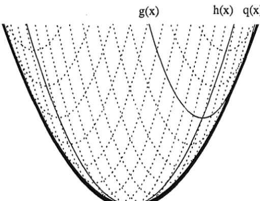
The following key lemma provides the details. It describes the effect of sliding the epigraph of one positive definite quadratic form along the graph of another. Fig. 3 illustrates this in the one dimensional case.

g(x) h(x) q(x)

I ' I I I I t

I I r 11 I f

f I f 1' I I t

[image:7.600.183.439.563.760.2]

(8)

Lemma 2 Let H and G be positive definite matrices. Let S = ( H

+

G)-1

and Q = HT sT GS H

+

GT ST HS G. The epigraph of the quadratic form xT Qx is obtained by sliding the epigraph of the quadratic form xT Gx along the graph of the quadratic form xT H x.

Proof:

Let g and h be the two quadratic forms represented by G and H respectively. Let

q(

x)

be the lower envelope obtained by sliding the graph of g along h. We now show q(

x)

is a quadratic form with the required matrix.

q(x)

=

min(g(x -y)

+

h(y))

y

=

mjn ((x -

Yl

G(x·-

y)

+

yT Hy)

Tal<lng derivatives with respect toy, the minimum occurs when 2G(x - y)

=

2H y. Since

H

and

G

are positive definite, the sum is invertible, thus y =

(H

+

G)-1Gx. Using this value for y, gives q(x) = xT Qx with Q

=

HTSTGSH

+

GTSTHSG as required. II

The following proposition shows that GPBA with Q from Lemma 2 and zero linear term can be used to give accelerated performance.

Proposition

2 Given a function f and positive definite matrices H and G as described. Let S

=

(H

+

G)-1 and Q = HTsTGSH

+

aTsTHSG. At each iteration calculate replacement values x'f __.:.Xi+ H-1\lj(xi) and r(xi)

=

J(xi)

+

~('Vf(xi)f

H-1\lf(xi)· An acceleration over both (1) and (2)

of proposition 1 is obtained by using the replacement values during the Update Envelope Function step of GPBA with Q and zero linear term.

Before providing the proof, it is worth looking at a few special cases. If

H

and

G

commute, the formula simplifies to Q

=

HG(H

+

G)-1. For H

=

B1I and G

=

BuI,

the formula gives Q =

BB~~

I. We state this special case and note that the replacement values are appropriate to1 othe; algorithms like [ 4] which use the same building blocks for the lower envelope.

Proposition

2' Given a function Jin the class Cf(Bz)

n

C~(Bu)

n

ZG. Let

B = B1Bu/(B1 +Bu)· An acceleration is obtained by using the -replacement values

xf

and

r(xi)

during the Update Envelope Function step of SPBA with Band zero linear

term. Here xf

=

x;

+

(1/

B

1) V'

f( x;) and

j"(

x;)

=

f( x;)

+

llY'

~~

1 •lll

2

.

The proof using the geometric ideas developed in [l] and [2] identifies a bigger region that can be removed.

(9)

Xi+ H-

1

Vf(xi)

and

fa(xi)

=

f(xi)

+

~('Vf(xi))TH-

1

Vf(xi)

as stated. During the Update Envelope Function step of GPBA with H, the function

hi(x)

is

f(xi)

+

Vf

(x - Xi) -

~h(x

- Xi)·

Expressed in terms of the replacement

values this is

fa(xi) -

~h(x

- xf).

Now

H

was chosen so

hi(x) :::; f(x).

So by proposition 3.2 of [2] at all points of the graph of

hi(x),

the regions below the translated graphs of -~g(x) can be removed, the union of these by Lemma 2 is the region below

r(xi) -

~q(x

- xi).

It is a paraboloid with maximum at

(xi' r(xi))

and contains the paraboloids used by the two methods mentioned in

Proposition 1. So using the replacement values for GPBA with

Q

and zero linear terms gives an acceleration over either method (1) or (2) of proposition 1. II

Figure 4 One dimensional illustration for proof of Proposition 2

3. Relation to other algorithms and accelerations

If a Lipschitz bound M is available, the accelerations given in [l] are compatible with proposition 21

•

[image:9.602.108.472.296.542.2]

(10)

Proposition

3

Given ajunctionf in the class C((B1)

n

C~(Bu)

n

L(M)

n

ZG. Let

B

=

B1Bu/(B1 +Bu)· An acceleration is obtained by using replacement values

xf and

fa(xi) during the Update Envelope Function step of SPBA with Band zero linear term.

Here

xf

=

Xi+ (l/B1)'7f(xi) and

a . _ {

f(xi)

+

ll'V~~/)!1

2

+

₂

!

₂

(di-li)

2

di> li

f

(xi) -

ll'Vf(xi)ll2

where

f

(Xi)

+

2B di ::::; li

-l 2

d·

=

f(x·) - a· and l·

=

M2 - ll'Vf(xi)ll

i i i ' 2B

2B1

Proof:

The paraboloid which is the region below the graph of

r(xi)

-~Bllx

-

xf

11

2

is removed during the ith step of

SPBA.

Using

xf

and

r(xi)

in place

Qf

Xi

and

f(xi)

in proposition 5 of [1] gives the result. •

Algorithms using a Lipschitz bound can modified to incorporate second derivative

bounds and use the gradient. The algorithm of Mladineo [5] deals with Lipschitz

continuous function in

L( M).

It is an algorithm in Piyavskii 's scheme with

hi (

x)

=

f(xi) -

Mllx -

Xiii

and for dimension one reduces to that of Piyavskii [6] and Shubert

[7].

Proposition

4

Given ajunction fin the class C((B1)

n

C~(Bu)

n

L(M)

n

ZG.

let B

=

B1Bu/(Br+ Bu)· When using the alg-orithm of Mladineo, an acceleration

using gradient information is obtained by using the replacement sample poinJ

::1

~;·(x:) :~:: ;;:,~::t:~::/:e{F=~:;:::t~l:;:::::•s :::g~n

f(xi)+

2B

+

2B d, - 2B

2 l

where d·

=

f(x·) - a·+

ll'Vf(xi)ll

i i i

2B1

Proof:

In the notation of [ 1] and using a slight extension of Lemma 2, it follows that the MB-parabolically capped cone with apex at

(xf,

r(xi))

could be removed during the ith step of Mladineo's algorithm. Using

xf

and

r(xi)

in place of

Xi

and

f( Xi)

in proposition 3 of [l] gives the result. 11111

4. Comparisons

The results of this paper provide accelerations in a one-step sense. For a given

iter-ation, using an acceleration always produces a better bracket than not using it. Since the sequence of sample points used by these algorithms is determined by using the

arg min

Fi(x)

at each step, using the accelerations will produce a different sequence

of sample points, so on occasion will perform worse. We explore the convergence

(11)

Testing

RATFOR implementations of SPBA and GPBA were run with the various modifications

for a number of standard test functions. Each iteration requires a function and gradient evaluation. Tests were stopped when both an absolute error measure was less than 0.01 and a relative measure was less than 0.0001. The tests of the acceleration of Mladineo's algorithm were carried out only by a discrete simulation (described in [2]). The particulars are summarized in Tables 1-4.

The standard test functions are described in [3]. To illustrate the differences between using G and H, variants a-d of EXP2 of the form

f(x,y)

=

-7re-1/2(ax2+b(y-e)2) _

( 2

2)

(1 -

7r)e-

1₁_{2 ex +d(y+e)} _{were used. EXP2 has circular contours, the variants have}

'"eliptical contours at the global minimum. EXP2b is highly curved at the global minimum. EXP2c and d have two local minimum. The contours around both these look similar for EXP2c while they are quite different for EXP2d. Table 5 gives details.

Test parameters Reference

L

=

vr

_i

L

=

0

L

=

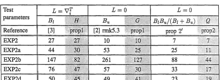
0

Table 1 ITERATIONS TO CONVERGENCE USING SPBA AND ITS ACCELERATIONS Heavier shaded columns from methods presented in earlier references.

Test

L=O

parameters

Bu B1Bu/(B1 +Bu)

Reference [3] [2] rmk5.3 prop 2'

EXP2 27 10 7

EXP2a 44 53 25

EXP2b 147 261

88

EXP2c 76 57 33

EXP2d 50 49 23

[image:11.602.82.517.355.513.2] [image:11.602.85.525.605.766.2]

(12)

Test Mladineo Mladineo [l] prop 4 prop 4

SPBA prop 3 8

COS2 39

RCOS 123

ow

282

C6

55

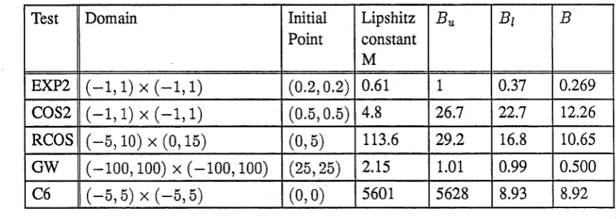
Table 3 ITERATIONS TO CONVERGENCE (DISCRETE TESTS) Heavier shaded column from method presented in earlier reference.

Test Domain Initial Lipshitz

Point constant M EXP2

(-1, 1)

x

(-1, 1)

(0.2, 0.2)

0.61 COS2

(-1,1)

x

(-1,1)

(0.5, 0.5)

4.8 RCOS

( -5, 10)

x

(0, 15)

(0,5)

113.6

ow

(-100, 100)

x

(-100, 100)

(25,25)

2.15

C6

( -5, 5)

x (

-5, 5)

(0,0)

5601

Table 4 Particulars -for test functions (best bounds used)

Test 7r a b c d e Bu B1

EXP2 1 1 1 .;

-

0 1 0.37

EXP2a 1 4 16

-

0 16 7.14

EXP2b 1 40 160

-

0 160 71.2

EXP2c .55 4 16 4 16 .5 8.77 6.51

EXP2d .55 4 16 16 4 .5 8.07 4.23

Bu 1 26.7 29.2 1.01 5628 7 34 100 283 79 Bz 0.37 22.7 16.8 0.99 8.93 G 1.0 I 1.0 D 10 D .58 D .82 D

Table 5 VARIANTS OF THE EXP FUNCTIONS (all using same initial point and domain as EXP2)

( note: D = diag(4,16), E = diag(9.4, 10.6) )

Comments

Five conclusions are apparent.

B 0.269 12.26 10.65 0.500 8.92 H

.37 I .446 D 4.45 D .407 D .399 E

• Proposition 2, 21 _{and 3 always provide substantial improvements. The} number of iterations in right hand columns of Tables 1 and 2 are often half the size of the corresponding entries in the first two columns.

[image:12.595.150.458.63.196.2] [image:12.595.69.519.256.416.2] [image:12.595.90.521.460.580.2]

(13)

• EXP2a and EXP2b reflect the differences in using G and H (rows 2 and 3 of Table 2). EXP2a is gently curved at the global minimum so using G is better than H, while EXP2b is strongly curved and H works better. • The use of the Lipschitz constant M (the darker halves of the columns in

Table 1) usually has no effect. Those accelerations using M take effect only if there is a large drop in value, and thus help only in the early stages of an algorithm. For RCOS and C6 this minimal drop is nearly the overall distance from minimum to maximum, so acceleration hardly occurred. For OW the minimal drop is quite small, the replacement values were often used, and the improvement is quite marked. Note sometimes these "accelerations" produced marginally poorer results. This is due to the fact that different sample sequences were produced. When repeated trials averaged over many different initial points were done, the accelerations were never worse.

• Both Mladineo's and the second author's algorithms when fully utilizing first and second derivative information give very similar results as shown by the similarity of columns 2 and 3 in Table 3

Concerning the discrete tests done for Mladineo's algorithm, note column 3 of Table 3 and the shaded part of column 3 of Table 1 test the same method. Likewise the heavily shaded results of Table 1 were done with discrete testing in [l]. The values are comparable and confirm that the discrete testing gives similar results to the actual running of the algorithms. The problem relates to differences in the stopping criterion. Discrete testing is appropriate for comparison testing shown in Table 3.

Conclusions and Future Directions

We have demonstrated two ways of improving the performance of some global optimiza-tion methods. The algorithms were easily modified to utilize fully both first and second derivative information.

A drawback of many methods that use bounds on first or second derivatives, including the ones presented here, concerns the calculation of the bounds. Finding good ones is often an equally difficult global optimization as the original. Work in this direction is needed. Local bounds appropriate to small regions in the domain are sometimes easier to obtain. So one area for future work appropriate to GBPA concerns incorporating subdivision of the domain, a modification that would readily lend itself to parallel computing.

References

[l] W. Baritompa, Accelerating Methods for Global Optimization, submitted

(14)

[2] W. Baritompa, Customizing methods for global optimization - a geomet-ric viewpoint, J. Global Optimization To appear

[3] Breiman & Cutler, A Deterministic Algorithm for Global Optimization,

Math. Program. To appear

[4] Yu. G. Evtushenko (1971), Numerical methods for finding global extrema (case of a non-uniform mesh), USSR Comp. Math. and Math. Phys. 11, 6,

1390-1403

[5] R. H. Mladineo (1986), An algorithm for finding the glbbal maximum of a multimodal, multivariate function, Math. Program. 34 188-200.

[6] S.A. Piyavskii (1972), An algorithm for finding the absolute extremum of a function, USSR Comp. Math. and Math. Phys. 12, 57-67

[7] Bruno 0. Shubert (1972), A sequential method seeking the global maxi-mum of a function, SIAM J. Numer. Anal. 9, 379-388