Remarks on the Erroneous Dispersion Surfaces from a
Pair of a Hyperbolic Branch and an Elliptical Arc of the
Intersected Two Laue Spheres Based on the Usual Crude
Approximation
Tetsuo Nakajima
Saitama Institute of Technology, Advanced Science Research Laboratory, Saitama, Japan E-mail: [email protected]
Received February 5, 2011; revised March 7, 2011; accepted March 8, 2011
Abstract
In almost all previous works, the hyperbolic dispersion surfaces of the central proper quadrics have been crudely derived from reduction of the degree from the bi-quadratic equation by use of some roughly inde-finable approximate relations. Moreover, neglecting the high symmetry of the hyperbola, both the branches have been approximated on the asymmetric surfaces composed of a pair of a branch of the hyperbola and a vertex of the ellipse without the presentation of reasonable evidence. Based upon the same dispersion sur-faces equation, a new original gapless dispersion sursur-faces could be rigorously introduced without crude omission of even a term in the bi-quadratic equation based upon usual analogy with the extended band theory of solid as the close approximation to the truth.
Keywords:Dynamical Theory of X-Ray Diffraction, Gapless Dispersion Surface, Gappy Dispersion Surface
1. Introduction
First of all, it could be necessarily considered that the firm establishment of E(energy) vs. k(wave number) curves as the dispersion relation of the electron in solids, which have been used as the usually popular gappy dis-persion surfaces by solid line in Figure 1 [1] in almost all works of the dynamical theory of X-ray diffraction (DTXD) [2-6], were carefully introduced from the solu-tions of the secular equation based upon the experimental and theoretical examinations in the low-energy elec-tron-diffraction by R. M. Stern et al. [1] and have pre-vented to foster greater understanding of DTXD. In the band theory of the solid state physics, the energy gap at the Brillouin zone boundary between the hyperbola and ellipse in Figure 1 could be introduced as a perturbative effect of the Fourier component of the periodic potential in the crystal [7], which is the off-diagonal term in the secular equation shown in the Section 5. It plays impor-tant role that the band structure and its electronic struc-ture occupied by electrons depending on their concentra-tion could give an insulator, a metal or a semiconductor and a semi-metal [7]. The energy band structure with the
forbidden band as the Bragg gap due to the potential bar-rier from the band theory in Figure 1 [1] could be valid for only the valence and conduction electrons and inci-dent electrons in the electron diffraction [1,7,10]. On the contrary, the off-diagonal terms of 2Cχ and 2Cχ
g g
K K in
Equation (2) in the Section 3 are composed of the wave number, the polarization factor and the Fourier compo-nent of polarizability as a response function of X-rays, which could be rewritten by χ λ2 π
g R Fg V [3]. Here
R is the classical radius of electron, λ the wavelength,
g
F the Fourier component of the structure factor and V the unit cell volume. All of the factors are transparent to X-rays contrary to the potential for electron, and there-fore cannot construct forbidden band as the Bragg gap, as in the Section 2 [8,9].
Secondly, the hyperbolic gappy dispersion surfaces in DXTD have been arranged near an intersectional point at the Lorentz point LD between the hyperbola and ellipse
Figure 1. The familiar dispersion surfaces. The formation of the Bragg gap has reasonably derived only in the elec-tron-diffraction by Stern [1]. Superposition of the hyper-bola over the gap between a branch of hyperhyper-bola and a vertex of ellipse in DTXD is a misapplication by a light-hearted interpretation.
central proper quadrics, the ellipse and hyperbola can be formed from the loci that the sum and difference of the two distances from the definite two points are constant, respectively, as is written like
2
21
x a y b . Therefore, the hyperbola has two asymptotes that cannot exist in the ellipse. Let it be ever so infinitesimal line elements in each, ellipse and hyperbola are invariably ellipse and hyperbola, respectively. Generally, approxi-mation can round off magnitude of the quantity but can-not change the plus and minus signs in algebra and the symmetry in geometry. Therefore, the ellipse could not transform into the hyperbola by approximation. By na-ture, that’s something that cannot be, as mentioned in the sections 3 and 4.
As a preliminary work, surpassing the above two er-roneous points the rightly reasonable dispersion surfaces [8,9] are carefully described based upon high analogy [3] with the extended band theory in solid state physics as the closest approximation to the truth [10].
2. The First New Gapless Dispersion
Surfaces in DTXD Based upon the Band
Theory of the Solid
Mainly following Kato’s scheme [2] based upon a man-ner of the Laue method [3], we carefully examined deri-vation of the gapless dispersion surfaces from the bi- quadratic equation of the two wave approximation. The vector propagation equation of an electro-magnetic wave by the electric displacement d in a medium with a peri-odic polarizability χ(r) has been represented by
2 rot rot 0
K χ
d d d .
Based upon this equation, the two wave propagation
equations from the Bloch waves of do and dgdefined by
doexp
i o
gexp
i g
d r k r d k r
could be derived to be
2 2
2 0o o g g
k k d K C d (1a) and
2 2 2
o 0
g g
K Cχ d k k dg (1b) in which k is the wave number in the crystal, K the wave number in vacuum defined by( 1 0
2
),
where n the refraction index, C the polarization factor and
χ kK nK
o, g
χ Fourier components of the polarizability, in which χ χg g χg2 from χg χ*g by neglecting the
absorption. Here, in order to solve the two wave propa-gation Equations (1a) and (1b), which could be repre-sented by the simultaneous linear equations with two unknowns, the necessary and sufficient condition, which is satisfied for existence of solutions [6] could be repre-sented by
2 2 2
o g 4 2 2
ij 2 2 2 o
k C
k k
C k g
g g
K χ
K χ
k
S k
k
2 k
0 2 2 4 2 2 o g K C χg ,
k k (2) which was designated as the bi-quadratic dispersion surface equation called by Pinsker [4], not the secular equation. Here, heads of ko and kg(kog where
g is thereciprocal lattice vector)in Figure 2 lie at the point O and G and their initial common point 1, which chanced to be there satisfies a loci in Equation (2) in the
[image:2.595.329.531.462.639.2]S
Figure 2. Diffraction in reciprocal space based upon the two wave approximation. The points S1 and S2 are intersectional points, through which a horizontal lines of H1 and H2 are
reference lies. The vector of OGg is the reciprocal lattice vector, S O1 ko
the incident wave vector and S G1 kg
reciprocal space.
The diagonal terms of S11 and S22 in Equation (2) rep-resent the two same radius circles intersected at two points S1 and S2 in Figure 2. The roots of X(k20: positive definite) in Equation (2) can be given by
2 2
2 2
2 4 2 2o o
1
4 .
2 g g
X K χ
k k k k C g (3)
Accurately, Equation (2) could not be a form of the secular equation but has been frequently impressed as the secular equation in some references [2,3,6]. Just to be sure, the intrinsic secular equation of equation (2) could be represented from the usual definition as follows:
2 2 22 2 2
Det ij
g
g g
k E K Cχ
K Cχ k E
k S E k o ij
2 2 2 2 2 2
O g 2 O g
E k E
k k k k
2 2
2 4
2
2 O g k k K Cχ 0,k k g (4) in which E is the eigen-value, 1 for
0 for ij i j i j
the
Kronecker’s delta, which represents the unit matrix. The eigen-values of Equation (4) could be obtained to be
22 2 2 2 2 4 2 2
o o
1
4
2 g g
E k K C χ ,
k k k k g
(5)
where the first term of “ ”in Equation (5) only trans-lates the origin of E, therefore ordinarily it is omitted hereafter. It is the most important that the behavior of the whole multinomial commonly in the right hand side in Equations (3) and (5) should be carefully analyzed over all k-space especially in the vicinity of the Brillouin zone boundary. When E = 0, Equations (2) and (3) are com-pletely equivalent to Equations (4) and (5), respectively. Then, it is self-evident that the analytic results in both of Equations (3) and (5) without any abbreviation of even a term as done in the conventional crude approximation could remain wholly valid as the close approximation to the truth. It could be understood that the refracted beam k in the roots in Equation (3) can be sufficiently character-ized by AM and FM due to the three kinds of photons of
o,
2 k
k kg and K,which could be polarized by the periodic
electron distribution in χg in conformity with the dual
polarized photons by C.
Approximately assuming that 4 2 2 0 two in-
g
K C χ ,
tersected circles with the same radii in Equation (3) are shownin Figure 2. If the magnitudes of ko and kg are
close to each other, then the term of 4 4 2 2
g
K C χ cannot be neglected. Thus, the amplitude of neither plane waves is negligible. When ko kg , Equation (3) becomes
2 2
o g
X k K C and hence the ratio of do to dg,
determined from Equation (2) is 2 2
g g
K Cχ : K C χ
Hence, d : do g 1 1: . Assuming that 4
2
2g
K Cχ is large compared with the first term under the radical sign in Equation (3) in case of 2
o 2
g
k k , X can be expanded to be,
2 2
2
o2 2
2 2 χ g K C o 1 8 2 g g gX k k K Cχ k k
(6)
If we translate the origin of k by g 2 and consider the vector k g 2 and if we denote by x the compo-nent of k parallel to g and byz the normal compo-nent to g, then by using the following relations, after more elaborate vector analysis than it looks like,
2 2 2 2
o 2 o
g ko
k k g g k
2 2 o 2 2 2 z g
x g g k x g
and
2
2 2 2 2
o 2 g
k z x z x x
2 4
g
g ,
a reasonable roots of X in Equation (3) from the 2nd and 3rd terms in Equation (6) can be rewritten as
2 2 2
4 X z x g
2 2 2 2 2 g g K C
K C
x
g (7) The 4th term in the brackets in Equation (7) could be the most important one expanded in series near the Brilluoin zone boundary described in the above as one of main subjects. As a result, the 4th term in Equation (7) could be indicated by
2 2 2 2 2 2
g g
K C K C
y g x . (8)
The expressions in Equation (8) show the precisely ca-nonical forms of the hyperbola and ellipse as
2 2 2 2 2
y b b x a
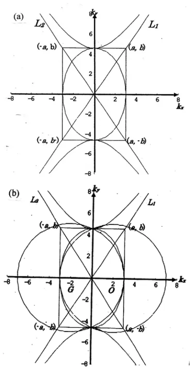
(9) in which the ellipse with plus sign and hyperbola with minus one are shown in Figures 3(a) and 3(b), together with asymptotes of y x 0b a labeled L1andL2 in
hyperbola. The constants a and b in Equation (9) can be given by Equation (8) as
2
2 g
Figure 3(a). The dispersion surfaces composed of the ellipse and hyperbola in Equation (8) with the two asymptotes L1 and L2 defined by extended two diago-nals of the rectangle with both sides of 2a and 2b. 3(b).This shows superposition of Figure 3(a) upon Figure 1, which shows smooth variations of the dis-persion surfaces in forward and backward X-ray near the Brillouin zone boundary.
χg
bK C . (10b) Therefore, 2 2 2 2
g
a K C g and 2b2K Cχg from Equations (10a) and (10b) are the minor and major axes of the ellipse, respectively and the latter of 2b also stands for the transverse axis of the hyperbola. The gra-dients of the two asymptotes of hyperbola defined by the gradients of diagonals of the rectangle with both sides of 2a and 2b in Figures 3(a) and 3(b) could be expressed by
b a 2CgsinB from Equations (8) and (9) by the Bragg law, which will be discussed in the final section. Both of the hyperbola and ellipse could stand in a line without a gap as in Figures 3(a) and 3(b).Conse-quently, it could be apparently proved that the expected Bragg gap as shown in Figure 1 between hyperbola and ellipse could not absolutely exist in Equation (8) in DTXD and the gappy dispersion surfaces in Figure 1 can be rigorously set to the right gapless dispersion surfaces in Figure 3(a).
3. Examination on the Crude Approximation
to Derive the Previous Gappy Dispersion
Surfaces
According to the previous works [2-6], the dispersion surface Equation (2) can be factorized as
2 2 2
2 2 2
χ
χg g
g
k K C
K C k
k
k
o
4 2 2χ 0g g
k k k k K C g
ko k ko k . (11)
In almost previous references [2-6], by use of the nu-merical approximate relations of
O 2 2
k k K k and kg k 2K2k, (12) the central proper bi-quadratic Equation (11) could be further decomposed into two quadratics as follows:
4 2g
k k K 0
ko k (13a)
2 2 2χ 4
0g g
k k K C
ko k . (13b)
The factorization in Equation (11) by Equation (12) is over the limits of approach and beyond reasonable con-ception in Equation (4).
Originally, the bi-quadratic dispersion surface Equation (2) should be a product of the two central proper quadrics consisting of the hyperbola and ellipse including circle as easily understood from Figures 1 and 2. First, the central proper quadric of the hyperbola in Equation (13a), which could be constructed by replacing a very big product of
O
k k and kgk with 4K2 by use of Equation (12), has been cut down without any thought for the conse-quence. Secondly, although a product of both terms of
kok and kgk has been approximated at zero from
Equation (12), an order of magnitudes of the second term in Equation 13(b) can be estimated to be
2 9to10
4 2 2 2 2 2 2 5 2
2 8to10
4 4 10 10
4 10 1
g g
K C χ K C χ C
C
.
[image:4.595.65.263.75.456.2]analysis of ko and kg considering its direction and
orientation in the vector space. These approximations are unmistakably self-contradictory and definitely break na-tive goodness of the two central proper composite quad-rics in Equation (2), which should be never allowed without rigorous verification. This is a violation without cause.
Reserving examination of the elimination of the de-composed factors in Equation (13a) in the crude ap-proximation, it could be concluded that Equation (13b) intuitively has at least two solutions. From the condition that the product of two variables is a constant of
2 2 2χ 4g
K C
in Equation (13b), a simple solution represents a rectangular hyperbola. However, this is not practically reasonable, considering the variations of the Bragg angle. In another solution, it could be easily un-derstood from a well-known attribute that the product of the two perpendiculars to the two asymptotes of the hy-perbola from an arbitrary point on it is constant described by
a b2 2
a2b2
, which could be easily prove from the canonical form of Equation (13b) as2
y x
B B
1 2cosθ 2sinθ
g g
k k
KC KC
2
,
0θBπ2 .
(14) The fitness of Equation (14) to the hyperbola at the cen-ture point D in Figure 1, which is composed of a hy-perbolic branch (named as “branch 1” forL
, k
o
k 0
g k
k ) and an elliptic arc near a vertex on the major axis side (similarly “branch 2” for ) has not yet been correctly examined from a geometrical viewpoint to decide whether to support Equation (13b) on the principle of being fair and just.
, g 0
kok k k
4. Geometrical Examination on the
Conventional Gappy Dispersion Surfaces
In DTXD
It is thoughtless beyond mathematical knowledge to as-similate both substantially different extremities from a different nature of symmetry between hyperbola and ellipse, by simple numerical approximation in Figure 1. In Figure 2, the oblique lines of T1 and T2 represent tan-gential lines of two circles at the intersection point S1. It is very important to note that the intersected curves above and below H1 show quietly an obvious asymmetry, which could be paraphrased as follows: the vertically opposite angles at the intersectional point S1 of the two composite arcs O1S1G1 and O2S1G2 defined by intersec-tional angle included by both of the tangential lines T1 and T2 at S1 are identical. The angle included by two tan-gential lines at the points O1 and G1 on both arcs S1O1and
S1G1 can increase with increasing distances to both points O1 and G1 from the point S1 and become mono-tonically larger than the vertically opposite angles in the vicinity of S1. But a variation of the corresponding angles included by two tangential lines at the points O2 and G2 on both arcs S1O2 and S1G2 can become entirely vice versa. As easily imagined from Figure 2, both of the whole closed curves of oval S1G2G3S2O3O2S1 and co-coon-shaped S1O1O4S2G4G1S1 constricted in the middle could be redrawn as hyperbolic and elliptic dispersion surfaces with the Bragg gap as in Figure 1 for low- energy electron-diffraction by Stern [1], not for X-ray diffraction. This is a rigorous proof of asymmetry of arcs O1S1G1 and O2S1G2, from which the symmetric branches of the hyperbola can never be constructed. Therefore, the gappy dispersion surfaces in Figure 1 cannot be applied to TDXD as the hyperbola. In the previous works, a pair of asymmetric arcs of O1S1G1 and O2S1G2 has been in-sensitively replaced by the hyperbola of Equation (13b). This is the second violation without cause. For a long term, the previous works [2-6] have been just an attempt to put together the indefinable hybrid dispersion surfaces composed of a pair of the hyperbolic branch and elliptic arc to lay basis for today’s TDXD. However, by nature that is something that cannot be. Consequently, ap-proximation can round off magnitude of the quantity but cannot substantially change the plus and minus sign and geometrical symmetry. Therefore, the ellipse could not transform into the hyperbola by reasonably scientific approximation, whose use is totally outrageous and should not be fundamentally permitted.
5. Origin of the Energy Gap in the Band
Theory of Solid and Brief
Characterization of the Off-Diagonal
Term in the Dispersion Surface Equation
(2)
There are very close resemblance in physical treatment between the energy gap in conduction band [1,7,10] and anomalous transmission of X-rays [2-6] but the definite necessary results reveal that the off-diagonal terms of the Fourier component of potential in electrons create a for-bidden energy gap [1,7,10] and those in photons in Equ-ation (2) closely relate with the different ratio between the absorption and transmission of photons [2-6].
According to Kittel [7], two different standing waves of electron in solids could be derived from the two trav-eling waves of expi x / a and exp
i x a
as
ψ exp i x exp i x 2cos x a
a a
and
i
ψ exp exp
2 sin
i x x
a a
i x a .
(15b)
The two standing waves
and ψ
pile up electrons at different regions, and therefore the two waves have different values of the potential energy. This is the origin of the energy gap. The probability density ρof a particle is equal to ψ ψ* ψ2
k
i
. For a pure traveling wave exp( x), ρ is equal to exp( x)exp(-ikx)=1 so that the charge density is constant in Figure 4(b).
k
i
From the standing waves ψ
in Equation (15a), the probability density could be expressed by
2 2
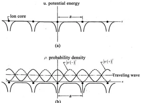
ρ ψ cos x a .The function piles up negative charge on the positive ions at the periodic lattice points of x = na (n = 0, 1, 2, ), where the potential energy is the lowest. For the standing wave
ψ in Equation (15b) the probability density is given by
2 2
ρ ψ sin πx a ,
which concentrate electrons away from the ion cores. Consequently, the wave function ψ
piles up elec-tronic charge on the cores of the positive ions, thereby lowering the potential energy in comparison with the average potential energy seen by a traveling wave in Figure 4(b). The wave function ψ
piles up charge in the region between the ions, thereby raising the poten-tial energy in comparison with that seen by a traveling wave in Figure 4(b). When the expectation values of the potential energy could be calculated over these threeFigure 4(a) Variation of electrostatic potential energy of conduction electron in the field of ion cores of a linear lat-tice. 4(b) Distribution of probability density ρin the lattice for ψ 2 sin2πx a (solid line), ψ 2cos2x a
charge distributions, it is in the nature of things that po-tenti ρ
trave
(dotted line) and for a traveling wave (one point broken line) [7].
al energy is lower than that of the traveling wave, whereas the potential energy of ρ
is higher than that of the ling wave. If energy difference be-tweenρ
and ρ
is equal to Eg, th an energygap of width becomes
en
g
E Assuming that the potential energy lectron in the crystal at the point x could be expressed by
in e
cos 2
U x U x a ,the energy difference between two sta ing wave states is
nd
12 2
d
E xU x
0
g
2 2
2 dxUcos 2 x a cos x a sin x a U
.It is found that the gap is equal to the Fourier comp ent of the crystal potential, which is the off-diagonal term in
on
the matrix
Sij in the secular Equation (4) and can cause an insulator, a metal, a semimetal etc in the above. In DTXD, by use of kgkog, the amplitudes of the Bloch waves in the section 2 [5] could be given by
oexp
i o
gexp
i g
d r d k r d k r
o gexp i
exp
i o
d d g r k r .
From this, the intensity of the wave-field can b given by e
2 2 2
o 1 2 cos
I d d R RC g r , (16) in which the amplitude ratio is represented by
g o o g g g
R d d CK CK (17)
where
2
o o o
α K 2 k k k 1χo
and
2
2
1
g g g
α K k k k χg
from off-diagonal term in the matrix
Sij g r
. For simplic-wave field
inten-
ity, instead of pile up of electrons, thesity is modulated by the factor cos
in Equation (16), which has maxima atg r n. It corresponds to an atomic plane and minima at g r
2n1 2
with in-tegral n. Therefore, by givi fferent reading r in-stead of x in Figure 4(b), the m ima of the standing wave occur at or halfway between the atomic planes. Including a role of the polarization factor C, it is important to stress that all of the off-diagonal terms in Equation (2) are transparent to X-rays as aforementioned and never construct the forbidden energy gaps in Figure 1 by splitting of the energy bands. The existence of the off-diagonal terms in Equation (2) could give energyng a di
axima and min
[image:6.595.59.285.482.648.2]transmission to absorption due to the photoelectric effect. For example, in the 200 reflection in NaCl, the structure factor Fg is positive. Hence, χgis negative and the
wave-field in branch 2 is absorbed more strongly than that in branch 1shown in Figure 5. The effect is well known as the Borrmann effect [5]
6. Results and Discussion
.
sion be c In DTXD, the asymmetric disper solid line in Figure 1 that could
surfaces shown by omposed of hyper-olic ch and elliptic arcs have been aggressively b bran
camouflaged with the gappy dispersion surfaces devised from the crude approximation beyond the fundamental algebra and geometry in Equation (13b) mentioned mainly the Sections 3 and 4 in which they have been constructed out of the quadratics crumbled from the bi-quadratic equation based upon the crude approximated relation in Equation (12). It means that these surfaces have been lacking fundamental consistency based upon the physical necessity. Therefore, the branch 2 has not the intrinsic asymptotes, because the root is from a part of the vertex of the ellipse. Hence, the previously wide-spread analyses in DTXD by use of Equation (13b) should be reexamined based upon the new gapless dis-persion surfaces in Figure 3(a) in Equation (7).
From Equation (14), another canonical form of the hyperbola in Equation (13b) could be represented as fol-lows,
2
2 2 2 2
2 k cosθ k sinθ 1 0, θ π 2 .
KC
y B x B
(1 racteristic that the in of the factor in the large value a entioned in the se 3 and the disp te
B
verse
quation (18) is equal to very ction
g
It is cha
first parentheses E s m
8)
ersive rms in the second factors consisting of two terns in parentheses are remarkably modulated by the sine squared θB plus cosine squared θB in Figure 6. In the region of 0θB π 4, the gradients of the hyperbola are steep and the intersectional angles of the asymptotes are the ac e angles. And the majo axis of the reference ellipse curve of 2 2
ycos θBsin θB1
k is parallel to the ky-axis. When
ut r
2
B π 4
θ , it becomes the rectangular hy- perbola and the reference curve is a circle. Moreover, in
B
π 4θ π 2, ntersectional angles become the obtuse angles. he offered ellipse for reference is
those i That of t
Whereas, from parallel to the kx-axis.
[image:7.595.319.531.241.450.2]Equation (9), the canonical form of the hyperbola and ellipse in Equation (8) could be repre-sented as
Figure 5. Intensity of the two wave-fields at the exact Bragg condition in the 200 refection. Note that branch 1 and 2
waves imum intensity and a m at th
ig
have a min aximum one e
atomic positions, which are analogous to the electrons in Figure 4(b).
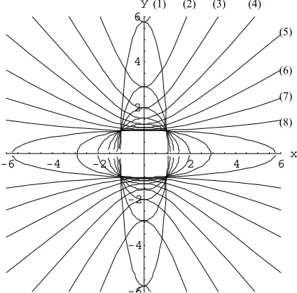
F ure 6. The main part of the dispersion surfaces of 2cos2 2sin2 1
ky θBkx θB in Equation (18), together with the pses of k2cos2 k2sin2 1
elli y θB x θB as a reference. The Bragg angles from (1) 10 to 8 (80) in every ten degree should be slope hyperbola to the gentry slope one in order.
assigned to the steep
2 2
y
k k
2 1 0 2 .
2 x
g g
, g k
K C K Cχ g
(19)
The major axis of ellipse in Equation (19) can b stantly parallel to the ky-axis because it is constant
ger than the minor axis like
e con-ly lar- 2
2K Cχg gK Cg since Kg in the order of magnitude in the region of
0 g 2k, which could corresponds to the region of the Bragg angles of 0B 2 in Figure 2. It is consid-ered that ppearance of the scattering vector a g only in the parameter a in Equation (9) could be appropriate. Further the gradient of the asymptotes of the hyperbola in Equation (19) can be represented as follows,
-6 -4 -2 2 4 6x
-6 -4 -2 2 4 6
y(1) (2) (3) (4)
(5)
(6)
) (7
(8)
b a 2 sin B gC
.
If the Bragg angle B is larger than 0 5. by a r
estimation of the a expression, t intersectional angles of the asymptotes could be the acute angle and reasonable.
rom
Dr. R. Negishi and the late ful stimulating discussions.
Prof. Dr. H. Kobaya
. References
] R. M. Stern, J. J. Perry and D. S. Boudreaux, Reviews of
8
ough Morden Physics, Vol. 41, 1969, pp. 275-295. [1
doi:10.1103/RevModPhys.41.275 [2] N. Kato,Kaisetsu and Sanran(in
bove he
Conclusively, it is very important to p ote that the afore-mentioned misapplication of Equitation (13b) should be reasonably set to rights and validity of the new proposed gapless dispersion surfaces in Equation (19) an
Japanese), “Diffraction
y Diffraction,”
rys-opography,”
Perga-tsu (in Japanese), “X-Ray
Dif-6th
Edi-ajima, ECM26, Darmstadt, 2010.
Physics,” Chapter and Scattering,” Chapter 9, Toyko, 1978.
[3] A. Authier, “Dynamical Theory of X-Ra
Chapter 4, Oxford university press, New York, 2001. [4] Z. G. Pinsker, “Dynamical Scattering of X-Rays in C
tals,” Springer-Verlag, Berlin, 1978. [5] B. K. Tanner, “X-Ray Diffraction T d should be strictly examined by thorough
investiga-tion.
7. Acknowledgments
The author would like cordially thanks to Prof. Dr. T. ukamachi, Associate Prof.
mon Press, Oxford, 1976. [6] S. Miyake,X sen no Kaise
fraction,” 3rd Edition, Chapter 5, Tokyo, 1988. [7] C. Kittel, “Introduction to Solid State Physics,”
tion, Chapter 7, John Wiley & Sons, Inc., New York, 1986.
[8] T. Nak F
M. Yoshizawa in SIT for use e is also indebted to Emeritus
H kawa [9] T. Nakajima, XTOP, Warwick, 2010.
of KEK for useful suggestion and drawings of Figures 2,
![Figure 1. The familiar dispersion surfaces. The formation of the Bragg gap has reasonably derived only in the elec-tron-diffraction by Stern [1]](https://thumb-us.123doks.com/thumbv2/123dok_us/9032806.399703/2.595.83.264.75.234/figure-familiar-dispersion-surfaces-formation-reasonably-derived-diffraction.webp)