Classical Quantum Field Theory Based on the Hypothesis of the Absolute Reference System

ISSN Print: 2327-4352

DOI: 10.4236/jamp.2019.74052 Apr. 3, 2019 747 Journal of Applied Mathematics and Physics

Classical Quantum Field Theory Based on the

Hypothesis of the Absolute Reference System

Konstantinos Patrinos

National Technical University of Athens, Athens, Greece

Abstract

The quantum field theory based on the hypothesis of the absolute reference system is a classical non-relativistic theory, which is compatible with current quantum theory. This conclusion arises when one compares the theoretical results of quantum electrodynamics using the basic principles of this hypo-thesis. Wave equation, which replaces this of Schrodinger, is the classical wave equation of a peculiar electromagnetic wave, derived from the study of particle structure.

Keywords

Particle Mechanics, Field Theory, Quantum Electrodynamics, Quantum Mechanics, Experimental Confirmation of Particle Dynamics

1. Introduction

According to the hypothesis of the absolute reference system [1], the wave-behavior of the particles is described by wave functions that are solutions of the classical differential equation of the electromagnetic wave and replace the corresponding solutions of the Schrodinger equation. These wave functions de-scribe real electromagnetic waves originating from the particle photonic struc-ture according to this hypothesis. The states of high energy particles come from the solutions of a modified Dirac equation, which is adapted to the classical per-ception of this hypothesis. In the first section, two issues of particle dynamics are discussed. One is the Compton effect, and the other is the experiment of Bertozzi, which is one of the historical experiments for confirmation one of the basic principle of the special theory of relativity. In the other sections, a study of the wave-behavior of the particles in quantum mechanics and quantum electrody-namics is discussed.

How to cite this paper: Patrinos, K. (2019) Classical Quantum Field Theory Based on the Hypothesis of the Absolute Reference System. Journal of Applied Mathematics and Physics, 7, 747-780.

https://doi.org/10.4236/jamp.2019.74052

Received: February 1, 2019 Accepted: March 31, 2019 Published: April 3, 2019

Copyright © 2019 by author(s) and Scientific Research Publishing Inc. This work is licensed under the Creative Commons Attribution International License (CC BY 4.0).

http://creativecommons.org/licenses/by/4.0/

DOI: 10.4236/jamp.2019.74052 748 Journal of Applied Mathematics and Physics

1.1. Compton Effect

We will examine now the scattering of a photon by an electron, in the reference system of the laboratory (which is the earth’s frame of reference), that is Comp-ton effect (ref. [2], paragraph 2.3.4, p. 44, Compton effect), from the point of view of the absolute reference system. We assume that the energy of the photon is hν and the mass of the electron at rest is m. At the level XY, the electron momentum vector forms an angle −ϕ with the axis X, whereas the direction of the photon forms an angle θ with the same axis.

Based on what we have mentioned before about the absorption of a high energy photon from a free electron, the phenomenon studied will be accompa-nied by an increase in the mass of the electron equal to the equivalent mass of a bound photon

(

)

( )

₂ 2

ph

m =h ν ν− ′ c _{(due to the difference in the frequency of}

the photon incident to the electron and the corresponding outgoing) and also by a kinetic energy absorption equal to:

(

)

1 4

e

E = hν ν− ′ (1.1)

The total energy of the outgoing photon after the impact is equal to h

ν

′ _and the kinetic energy of the electron after the impact, as previously described, is equal to

(

)

2 2 ₂

e ph

E = m m+ γ u _{. The velocity u is measured with the} instru-ments of the frame of reference of the laboratory and the contraction factor is

(

_{2 2}

)

1 2

1 u c

γ

= − − _{. The momentums of the incident and outgoing photons will} be h

ν

( )

2c and h

ν

′

( )

2c _{respectively; the momentum of the electron is p,} while the frequency of the deposited mass of the bound photon is equal to

(

ν ν

− ′

)

2.

Due to the conservation of momentum on the X axis, the following relation is taken:

cos cos

2 2

h h _p

c c

ν ν′ _{θ ϕ}

= + (1.2)

The conservation of the momentum on the Y axis:

0 sin sin

2

h _p

c

ν′ _{θ ϕ}

= − _(1.3)

Of these two last relations:

(

)

(

)

2 2

2 2

2 1 cos 2

4 2

h h

p

c ν ν′ νν′ θ c

= − + − (1.4)

According to the previous mentioned and the relation (1.1):

(

)

2

(

)

2

(

)

2

2 2 2

2 1

2 4

ph

h

p m m u mh

c

ν ν

γ

ν ν

′ − ′

= + = − + _(1.5)

From these two latter relations, the change in the wavelength of the photon initially incident to the electron is calculated:

(

1 cos

)

c c h

mc

λ λ θ

ν ν

′ − = − = −

DOI: 10.4236/jamp.2019.74052 749 Journal of Applied Mathematics and Physics

1.2. The Experiment of W. Bertozzi

An experiment of controlling the correctness of a proposed dynamics, such as the dynamics of the absolute reference system, is that of W. Bertozzi1_{, which was}

carried out in the early 1960s, and refers to the measurement of the maximum speed of high energy electrons by a linear accelerator (ref. [4], chapter 1, De-partures from Newtonian dynamics, “THE ULTIMATE SPEED”). The al-ready accelerated electrons are released in small bundles (of time duration about

9

3 10 sec_× − _{), directed to the high-voltage negative end of the Van de Graaff}

ac-celerator. The path is described as “8.4 meter drift space” in Figure 1. Insulated leads at the ends of the path, collect the electrical signals of the beam.

These electrical signals are transmitted on a down-turn oscilloscope via two wires of the same length (so that the signals need equal time to reach the oscil-loscope). In this way the pulses displayed on the oscillator give the real time of transmission of the electron beam along the “drift space”.

While electron velocity measurements are determined directly using the os-cilloscope, kinetic energy is determined from potential difference produced in the Van de Graaff generator and electric field in Linac. This is a strictly prede-termined procedure, which has been tested in the laboratory by magnetic deflec-tion methods.

To test any dependency of the electron velocity from the force exerted, due to the very strong electric field, an additional measurement acquired by the high energy electrons is made to a further embodiment comprising an aluminum disk on which impinge the electrons at the end of their path and a thermocouple to measure the temperature increase of the aluminum disc, so the added energy in the form of heat will be proportional to the increase in temperature. In addition, an additional device for measuring the charge collected in the disk is used, in this way to determine the energy transferred from each electron. Such energy measurements were made in the estimated accelerator energies at 1.5 MeV and 4.5 MeV (tested by the above-mentioned magnetic deflection methods), whereby the corresponding values, obtained with the heat increase measurement method in the aluminum disc, were 1.6 MeV and 4.8 MeV.

The results of the experiment, listed in Table 1, are five measurements of the electron velocity at corresponding kinetic energy values.

The comparison of experimental results with theoretical calculations of the special theory of relativity and of the hypothesis of the absolute reference system, is certainly the basic criterion of convergence of the experiment with these con-siderations. The theoretical values of kinetic energy of the special theory of rela-tivity derive from the relation:

(

₁

)

2

rel

E =m γ − c (1.7) where m is the mass of the electron, u the electron velocity of the beam and

(

_{2 2}

)

1 2

1 u c

γ

= − − _{. The corresponding theoretical values of the hypothesis of the}

1_{The Ultimate Speed, W. Bertozzi, Education Development Center, Newton, Mass. 1962. For more}

DOI: 10.4236/jamp.2019.74052 750 Journal of Applied Mathematics and Physics

absolute reference system are taken from the relation:

2 2 1 2

abs

[image:4.595.209.536.279.504.2]

E = m uγ (1.8) However, the transferred kinetic energy in the target molecules, i.e. the expe-rimentally measured heat, is calculated based on the relative description of the electron collisions of the beam with the atoms of the material. In the absorbtion of a free high energy photon (i.e. of an, elementary, plane electromagnetic wave) from an electron, half of this energy is transferred as kinetic energy, while the other half is available for formation of additional elementary mass. Indeed, in the collision of the beam electrons with the target, the predominant image of the interactions is that of the polarized photons, as an image of elementary plane-waves, that act as interaction photons. Under these conditions the kinetic energy transferred to the target atom, in the form of heat, will be equal to:

Figure 1. The apparatus schematic diagram of measuring of the electron experimental flight time and of the electrons energy. The electrons have already accelerated due to the existence of a strong electric field of the Van de Graaff generator.

Table 1. Experimental results of W. Bertozzi’s measurements, as set out in his work en-titled “The Ultimate Speed”, in 1964.

kinetic flight electron

energy time velocity

K, MeV _{t, 10 sec×} −8 _{u, 10 m sec×} 8 _u2_{, 10 m sec×} 16 2 2

0.5 3.23 2.60 6.8

1.0 3.08 2.73 7.5

1.5 2.92 2.88 8.3

4.5 2.84 2.96 8.8

[image:4.595.195.539.595.738.2]

DOI: 10.4236/jamp.2019.74052 751 Journal of Applied Mathematics and Physics

2 2 1 4

abs

E = m uγ (1.9)

[image:5.595.209.540.574.694.2]

In an intermediate state, where the electrons of the beam move at speeds that are not very close to the velocity of light in the vacuum, a part of the total num-ber of force carriers will transfer the total kinetic energy to the target atoms, while the remaining force carriers the half of the kinetic energy. In this case, the energy transferred in the form of heat to the target atom will have a value be-tween

( )

_{1 4 m uγ}2 2 _and

( )

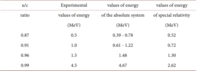
_{1 2 m uγ}2 2_.

Table 2 includes in the first column the ratio of speeds u c, in the second column the experimental values of the heat of the target, while in the third and fourth column the corresponding theoretical values derived from hypothesis of the absolute system and the special theory of relativity respectively.

The values of the first two lines in the table correspond to speeds equals to 87% and 91% of the light velocity in the vacuum, not so close to 100%. Since, accord-ing to the hypothesis of the absolute reference system, the heat transferred to the target has values between

( )

_{1 4 m uγ}2 2 _and

( )

_{1 2 m uγ}2 2_{, corresponding values}

are those listed in Table 2. Therefore, the experimental values are indeed within those ranges. The values of the last two lines of the table correspond to velocities very close to the speed of light in the vacuum, and according to the above, the corresponding calculated atomic heat is equal to

( )

_{1 4 m uγ}2 2_{. These high energy}

values are, as shown in Table 2, equal to 1.48 MeV and 4.67 MeV, with a small difference from the corresponding experimental ones. This is a confirmation of the hypothesis of the absolute system2_.

The theoretical values derived from the special theory of relativity are con-firmed only in the first line of the table, while the rest are much smaller than the corresponding experimental ones. These values might be somewhat acceptable if they were larger than the corresponding experimental ones. Therefore the expe-rimental results are in accordance with the special theory of relativity only in that the higher speed in nature is that of the velocity of light in the vacuum. However, it is not in agreement with the corresponding experimental values of energy.

Table 2. Table of experimental and theoretical values of the special theory of relativity and absolute reference system.

u/c Experimental values of energy values of energy

ratio values of energy of the absolute system of special relativity

(MeV) (MeV) (MeV)

0.87 0.5 0.39 - 0.78 0.52

0.91 1.0 0.61 - 1.22 0.72

0.96 1.5 1.48 1.30

0.99 4.5 4.67 2.62

2_{About experimental confirmation of particle dynamics from the point of view of the hypothesis of}

DOI: 10.4236/jamp.2019.74052 752 Journal of Applied Mathematics and Physics

2. The Wave Behavior of Particles

If photons are the structural component of matter, then a self-evident conclu-sion is that particle movements should obey a wave equation similar to the dif-ferential equation of the electromagnetic wave. It seems, according to the relative theoretical analysis of this section, in the light of the hypothesis of the absolute reference system, that the theoretical results of this assumption are acceptable, since they are in accordance with those of modern physics.

2.1. Particle-Frequency and Wavelength

A particle, as previously described, is composed of a number of bound photons and its total energy will be determined as the sum of total energies of these tons. The total energy derived from the mass frequencies of all the bound pho-tons of the particle shall be equal to:

2 0

1

1 1

2 2 i

N c i

E mc h ν

=

= =

∑

(2.1)

where

ν

c_i is the mass frequency of the i bound photon, 1 i

N c i=

ν

∑

is the sum of all mass frequencies and N is the number of bound photons. This latter equation results from the relation ( ) ( ) 2

1 2 hν_ci = 1 2 m c_phi , so _{1 1} 2 2

i i

N N

c ph

i=

ν

= i= m c h mc h=

∑

∑

.

We also accept, especially for very small particles (e.g., electrons), that the mass frequencies of the bound photons (which are similar to energy levels of atomic electrons) are different each other. The total energy of the particle will be:

(

)

2 2

1

1 1

2 2 i i

N

tot c u

i

E m cγ h ν ν

=

= =

∑

+ (2.2)

where

_γ

_{= −}

(

_{1 u c}2 2

)

−1 2 _{and u is the velocity of the particle measured by the}

measuring instruments of the laboratory inertial frame. We also assume that the total frequency of the i bound photon is equal to

ν

c_i +

ν

u_i, where νui is the

transfer frequency of the i bound photon.

The kinetic energy of the particle will result from the difference:

2 2 0

1

1 1

2 2 i

N kin tot u

i

E E E m uγ h ν

=

= − = =

∑

(2.3)

We define the quantity 1 i

N

q i u

ν

=

∑

₌

ν

_{as particle transfer frequency or simply}

as a particle frequency. Accordingly, the transfer frequency of the i bound pho-ton will be equal to the amount 2 2

i i

u mph u h

ν = γ _{, and since} 2

i i

ph c

m =hν c _,

the frequencies ratio is:

2 2 2

i i

u c

u c

ν _γ

ν = (2.4)

par-DOI: 10.4236/jamp.2019.74052 753 Journal of Applied Mathematics and Physics

ticle and is a characteristic of its reference system.

Therefore the kinetic energy in relation to the particle frequency is:

2 2

1 1

2 2

kin q

E = m uγ = hν (2.5)

Also the corresponding particle wavelength λ is determined by the relation

q

u

γ =ν λ. Therefore, the momentum of the particle is:

p=_k _(2.6) where k (the wavenumber) is equal to 2π λ.

2.2. Wave Function of a Free Particle

The wave function Ψ

( )

r,t of a free electron must obey, according to the abso-lute system hypothesis, not in the Schrodinger equation but in the differential equation of an peculiar electromagnetic wave:

( )

2

( )

2

2 2 2

, 1

,t t 0

u t

γ

∂ Ψ

∇ Ψ − =

∂

r

r (2.7)

which propagates at a velocity γu, and not at the velocity of propagation of the light in the vacuum.

This wave function as a solution of the wave equation will be of the form3_:

( )

( 2π ) ( 2 )

, ei _qt ei E tkin

t A ⋅ − ν A ⋅ −

Ψ r = r k =  p r _(2.8)

where the constant A is the amplitude of the particle wave,

( )

_{1 2} 2 2

kin

E = m uγ ,

ph

p m= γu _and

γ

= −

(

1 u c2 2

)

−1 2_{. If we define the operators of momentum} and energy with relations:

ˆ

p= − ∇i_{ (2.9)}

ˆ 2 kin i

E

t ∂ =

∂

 _(2.10)

the equation of momentum in relation to energy for a free particle

( )

2 kin

p= E

γ

u is equivalent to the equation:

( )

(

)

2

( )

2

2 2

1 _ˆ

ˆ , 2 kin ,

p t E t

u γ

Ψ r = Ψ r (2.11)

which is the aforementioned differential wave equation.

The operator of momentum is the same as that of the Schrodinger quantum mechanics, but the operator of energy is differentiated by a factor equal to 1/2, since the operator of energy of the Schrodinger quantum mechanics is equal to

ˆ

E i t ∂ =

∂

 .

If the constant A of the solution of the differential equation of electromagnetic wave is the electric field amplitude derived from the sum of all the electric fields of all the elemental photonic electromagnetic waves accompanying the

move-3_{ref. [6], Chapter 7, Plane Electromagnetic Waves and Wave Propagation, section 7.1, Plane}

DOI: 10.4236/jamp.2019.74052 754 Journal of Applied Mathematics and Physics

ment of the particle, then the quantity A2 _{is proportional to the energy density of}

these electric fields, and also it is proportional to the density of the mass inside the particle-space. Since the amount of this energy is constant for each particle, in a parallel beam of same particles with the same number of bound photons per particle, the magnitude

0

2 d

V Ψ V

∫

will be proportional to the number of par-ticles in the volume V0.

The particle current corresponding to the wave function Ψ

( )

r,t will result from the free particle wave Equation (2.7). By multiplying both members of this equation with _Ψ* _{and also writing the conjugate expression, we have the}

rela-tions:

2

* * 2

2 2 2

1

u t

γ

∂ Ψ

Ψ = Ψ ∇ Ψ ∂

2 *

2 *

2 2 2

1

u t

γ

∂ Ψ

Ψ = Ψ∇ Ψ ∂

and therefore:

*

* * *

2 2 ₂

2

i i

t m u

γ

t t m

  

∂ _Ψ ∂Ψ_{− Ψ}∂Ψ _{= −∇} _{Ψ∇Ψ − Ψ ∇Ψ}

    

 

∂   ∂ ∂   

  _(2.12)

so, based on the continuity equation 0

t ρ

∂ _{+ ∇ ⋅ =}

∂ j , we have got: *

* 2 2 2

i

t t

m u

ρ γ

 ∂Ψ ∂Ψ 

= _Ψ − Ψ _

∂ ∂

 

 _(2.13)

(

* *

)

2

i m

= Ψ∇Ψ − Ψ ∇Ψ

j  (2.14)

According to relations EˆkinΨ =

(

i 2

)

∂Ψ ∂ =t EkinΨ, pˆΨ = − ∇Ψ = Ψi p ,

( )

_{1 2} 2 2

kin

E = m uγ , p=mγu, for low speeds the following relations arise:

*

ρ

= ΨΨ _(2.15)

*

m ργ

= pΨΨ =

j u (2.16)

When the particle moves within a potential, then as we shall see later, the so-lution of the differential equation will surely vary as compared to that of the free particle. In this case, for a plurality of same particles, under the influence of this potential, the quantity

0

2 d

V Ψ V

∫

will also be proportional to the number of particles in the volume V0. For one particle the quantity

( )

2

ψ r is propor-tional to the density of mass on the location r of the particle-space. Therefore, the wave function Ψ

( )

r,t has a different interpretation from that of the cor-responding Schrodinger wave function, since it is classical and is a solution not of the Schrodinger equation but of the above-mentioned differential equation of electromagnetic wave.

equ-DOI: 10.4236/jamp.2019.74052 755 Journal of Applied Mathematics and Physics

ation, which are used in the case where the velocity of the particle is comparable to the velocity of light in the vacuum, are acceptable by the hypothesis of the absolute reference system. All the theoretical results of quantum field theory (for example, the theoretical results of quantum electrodynamics) are accepted by the hypothesis of the absolute system, if interpreted in the basis of this theory.

2.3. Wave Function of a Particle in the Presence of an External

Potential

Starting from the assumption that an initially free charged particle, for example a free electron or a parallel electron beam, enters a space with stable electrical po-tential, with some initial conditions of the problem, we reach a differential equa-tion. The solution of this equation gives the ability to determine the number of particles, as a function of the location. If the dynamic energy V of an electron is positive but less than the initial kinetic energy T, then the kinetic energy in the space of existing potential is Tp = −T V and the wave differential equation is

described in the previous subsection. When the dynamic energy is greater than the initial kinetic energy, then the kinetic energy Tp is negative, while the

cor-responding momentum value p= 2mTp is imaginary and the corresponding

solutions of the wave equation are exponential functions. Relative examples are those of the subsections 3.5 and 3.6. This is indeed a mathematical representa-tion of a natural absorprepresenta-tion phenomenon such as the propagarepresenta-tion of an electro-magnetic wave into a conductor (reference [7], CHAPTER XIII, OPTICS OF METALS, paragraph 13.1, WAVE PROPAGATION IN A CONDUCTOR), where the values of wavelength and refractive index are complex. This whole image shows a particle wave behavior similar to that of reflection, refraction, or absorption of an electromagnetic wave, that is, a beam of free photons incident to a material that may be reflective, transparent or absorbent.

The equations to which it generally obeys a particle motion to an external po-tential V is the energy conservation equation E T V= + and the differential equation of the particle wave. This differential wave-equation results from the equation of kinetic energy determination _{E V T− = = p}2

( )

_{2m , making use of}

the operator pˆ= − ∇i_{ , as in the previous subsection. The corresponding} diffe-rential equation, in the case of a particle whose total energy is constant (time-independent), is the same as that of Schrodinger:

( )

(

( )

)

( )

2

2 ₀

2m E V

− _{∇ Ψ − − Ψ =}

r r r

 _(2.17)

By including the time evolution of this particle’s state, we arrive at a more gen-eral form of the wave function, _Ψ

( )

_r,_{t = Ψ}

( )

_r ei(2πνqt)_{, where 2π 2}

q T

ν =ω= _.

This wave function satisfies the last differential equation, but also that which results from the relation _p2₌

(

₁

(

_γ2 2_u

)

)

( )

_2T 2 _{and from the operator}

(

)(

)

ˆ ₂

T = i ∂ ∂t and is the following:

( )

(

( )

)

( )

2 2

2 2 2 , , 0

2m u t

γ

t E V t

− ∂ _{Ψ − − Ψ =}

∂ r r r

DOI: 10.4236/jamp.2019.74052 756 Journal of Applied Mathematics and Physics

It also, of course, satisfies the wave-equation:

( )

2

( )

2

2 2 2 1

,t ,t 0

u t

γ

∂

∇ Ψ − Ψ =

∂

r r (2.19)

2.4. Particle Motion in Closed Orbits

For an electron moving in an atomic scale space, under the influence of the Coulomb field, the corresponding force exerted on it will have values that cor-respond to the same scale (that is, this force can not be enormous), and therefore, its velocity will not be comparable to the speed of light in the vacuum. So, the calculated contraction factor value is very close to 1 (γ 1). Such examples that will be studied in the next section are those of an electron in a hydrogen atom, the example of the potential of harmonic oscillator, and the example of an elec-tron moving periodically inside an infinite potential well.

According to mentioned in the previous subsection 2.1 about the kinetic energy in relation to particle frequency, according to the relation (2.5) presented in subsection 2.1 the frequency of the particle is proportional to kinetic energy. Therefore, in a closed periodic motion of an electron, the average value of the kinetic energy, over a time period equal to that required for a complete closed orbit of the particle, will be proportional to the average value of this frequency. This results in the following relation:

2

1 1

2 2

kin q

E = mu = hν _(2.20)

where Ekin, u2 , νq are time average values of kinetic energy, of velocity

squared, and of particle frequency respectively. A particular definition, which could be used in the consideration of wave motion of the electron, is that of an “equivalent particle-wavelength” according to the relation:

2

q q

u

λ ν

= (2.21)

and respectively is defined as “equivalent time period of oscillation” of the par-ticle-wave the amount Tq, calculated as following :

1 q

q

T ν

= (2.22)

Since the electron must behave, based on its structure, like a wave, in order for the movement of its closed orbit to be stable, this wave should be a stationary wave. Therefore, an additional binding condition is introduced which governs the periodic motion under consideration and is that thelengthoftheclosed or-bitshouldbeanintegermultipleoftheequivalentparticle-wavelength.

If the n length of the closed orbit is equal to nλq, where n is an integer,

then the time Tn of a closed path is equal to nTq and therefore the frequency

1 n Tn

ν = is related to the corresponding mean particle frequency:

q n n

DOI: 10.4236/jamp.2019.74052 757 Journal of Applied Mathematics and Physics

and finally a general equation is:

2

1 1

2 2

kin n

E = mu = hnν _(2.23)

This result, taking into account the equation of motion of the electron, ac-cording to the relative examples exposed in the next section, leads to the conclu-sion that the energy of the electron and also all physical quantities involved in this problem are quantized.

2.5. Uncertainty Principle

In the subsection 2.2 it is stated that the quantity ψ

( )

r 2 is proportional to the density of the mass in the space of the particle. This density is proportional to the number of bound photons per unit volume. Because a particle is located in a small area, rather than a single point, the location of the particle can be consi-dered as the point where the density is maximized. While the density distribu-tion of the particle mass appears to be continuous according to the funcdistribu-tion

( )

2

ψ r , it is distinct since the particle consists of a number of bound photons. The limits up to which the particle mass extends are those points in which, in a volume δV equal to the volume of the smallest bound photon, there is a calcu-lated mass (proportional to the amount of

_∫

_δV

ψ

( )

r 2dV) smaller than the mass of the same bound photon.

By normalizing the function

ψ

( )

r so that the integral in the infinite space is equal to the unit according to the relation:

( )

2 3_{d 1} ψ

∞ ∞ ∞

−∞ −∞ −∞ =

∫ ∫ ∫

r r (2.24)

the amount 2 2 2

( )

1 1 1

2 d d d

x y z

x y z ψ x y z

∫ ∫ ∫

r is the fraction of the unit which is equal to the ratio δm m_{, where} δm is the mass inside the volume 2 2 2

1 1 1d d d

x y z x y z x y z

∫ ∫ ∫

and m is the mass of the particle.

The mathematical development of the subject here was done by Andre Kess-ler4_{. It turns out that the Fourier conjugate of a very localized waveform will be}

spread out. Thus, if position and momentum (or energy and time, etc.) are Fourier conjugates, and if you know the position to a high degree of accuracy, then you don’t know the momentum very well and vice versa.

If

ψ

( )

r is the spatial part of the wave function, then this can be written in the form of a Fourier transform as follows:

( )

( )

3

( )

3

1 _{e d}

2π

i

ψ ∞ ∞ ∞ ⋅

−∞ −∞ −∞

=

_{∫ ∫ ∫}

Ψ k r

r k r (2.25)

The inverse Fourier transform is:

( )

( )

3

( )

3

1 _{e d}

2π

i

ψ

∞ ∞ ∞ _{− ⋅}

−∞ −∞ −∞

Ψ _k =

_{∫ ∫ ∫}

_r k r _{k (2.26)}

4_{“Derivation of the Heisenberg Uncertainty Principle’’, Andre Kessler, Department of Mathematics,}

DOI: 10.4236/jamp.2019.74052 758 Journal of Applied Mathematics and Physics

The momentum will be given by the relation p=k. We should expect the classical momentum to be the average value, and other values to be less probable. The corresponding probability will be expressed with a normal distribution. This implies that:

( )2

( )

2

0 2

e

P =A − −k k σk

k k (2.27)

where k0 the average value of wave number k, and σk is the standard

devia-tion. Therefore:

( )

_{P A e}− −( 0)2

( )

4σ2

Ψ = = k k k

k k

k (2.28)

Like earlier, we should expect the classical position to be the average value, and other values to be less probable, and therefore the probability of position is expressed by a normal distribution. If we let r0 be the most likely position for

the particle, then a normal distribution of the positions is:

( )2

( )

2

0 2

e

P A= − −r r σr

r r (2.29)

where r0 is the average position value, and σr is the corresponding standard

deviation.

Since the function Pr is the upper envelope of the function

( )

2 ψ r , the envelope of the function

ψ

( )

r is:

( )

_e( 0)2

( )

4 2

env P A

σ

ψ = = − −r r r

r r

r (2.30)

The coefficients Ar and Ak are calculated by simply normalizing the

nor-mal distribution:

3 3

d d 1

P P

∞ ∞ ∞ ∞ ∞ ∞

−∞ −∞ −∞ = −∞ −∞ −∞ =

∫ ∫ ∫

r r

∫ ∫ ∫

k k

this gets us:

(

)

3

(

)

3

1 _, 1

2π 2π

A A

σ σ

= =

r k

r k

Since the

ψ

( )

r _env and Ψ

( )

k functions are finally functions of r r− 0 and 0

−

k k respectively the Fourier transforms can be rewritten as follows:

( )

( )

3

( )

( 0) ( 0) 3

1 _{e d}

2π

i env

ψ ∞ ∞ ∞ − ⋅ −

−∞ −∞ −∞

=

_{∫ ∫ ∫}

Ψ k k r r

r k k (2.31)

( )

( )

3

( )

( 0) ( 0) 3

1 _{e d}

2π

i env

ψ

∞ ∞ ∞ _{− − ⋅ −}

−∞ −∞ −∞

Ψ _k =

_{∫ ∫ ∫}

_r k k r r _{r (2.32)}

After the integration of the second member of the last equation, the following equation is taken:

(

)

( )

( )

( )

( )

2 2 _{2 2}

0 0

3 4

3 3

2 2π

1 _e 1 _e

2π 2π

2π

σ σ _σ

σ σ

− − _ _{ − −}

=

 

 

k _r

k k r k k

r k

DOI: 10.4236/jamp.2019.74052 759 Journal of Applied Mathematics and Physics

In the last equation, the coefficients and exhibitors must be equal. The two equations:

(

)

( )

(

)

3 2 _{3 2}

2 ₂ 2 ₂

0 0

2

1 _{, 4}

2π 2π

σ _{σ σ}

σ

  _{ }

= − − = − −

   

  _{ }

 

r

k r

k

k k k k

end up in exactly the same relation:

1 2

σ σ_{k r} = _(2.34)

Due to the relation k p= , the standard deviation of the position in rela-tion to the standard deviarela-tion of the momentum is σ_r=σ_{p . Therefore:}

2

σ σ_{p r} = (2.35)

This, of course, the latter is true only if the probability distribution is normal. If it isn’t σ σ_{p r} will be greater, as the normal distribution turns out to have the minimum possible product. Therefore, in the general case:

2

σ σ_{p r} ≥ _(2.36)

or else:

2

∆ ∆ ≥p r  (2.37)

This is the Heisenberg uncertainty principle for position and momentum. The time-dependent part of wave function

ψ

( )

t can be written in the form of a Fourier transform as follows:

( )

1

( )

e d 2π

i t

t ω

ψ =

_∫

_−∞∞Ψ ω ω (2.38)

The inverse Fourier transform can be written as follows:

( )

1

( )

e d 2π

i t

t ω t

ω ∞ψ −

−∞

Ψ =

_∫

(2.39)

here the quantity ω

( )

2π is considered equal to the particle frequency νq, as

defined in the previous subsections. By following the same process as that of the spatial part of the wave function, using a normal distribution of frequencies and times, we arrive at the following relation:

1 2

t

ω

σ σ = (2.40)

where ω=2πνq. Also kinetic energy is given by relation Ekin=

( )

1 2 

ω

. So,

the last relation can be written as follows:

4

kin

E t

∆ ∆ = _(2.41)

As above, in the general case:

4

kin

E t

DOI: 10.4236/jamp.2019.74052 760 Journal of Applied Mathematics and Physics

In the case of a harmonic oscillator the total energy is equal to E=

ω

and therefore:

2 E t

∆ ∆ ≥ _(2.43)

This last relation is the Heisenberg uncertainty principle for energy and time.

3. Examples of Electron Motion in Various Potentials

We will then look at some of the best-known examples of quantum mechanics in the light of the hypothesis of the absolute reference system. The results obtained by solving these examples seem to be fully in agreement with the corresponding results of Schrodinger’s quantum mechanics.

If we consider as initial condition the relation γ1, and γ is denoted by the contraction factor of the particle’s reference system, then the expressions for the energy, momentum, etc, are that of Newtonian physics. Under this condition, the equations of the motions and the energies of electrons, in a good approach, are those of Newtonian mechanics.

3.1. Circular Motion of Electron in Coulomb Potential

A simplified example of an electron’s motion in a Coulomb field is that of circu-lar motion. In this case the field comes from a unique proton. In the general case, such as the Hydrogen atom, the orbit of the electron is elliptical, but this subject will be examined in a next example.

The total energy of the electron in our example is:

2 2 1 2

e E mu

r

= − (3.1)

where m is the mass, u is the electron velocity, e is the elementary charge, and r

is the position of the electron in a cartesian coordinate system, with origin the center of mass of the proton-electron system. Based on the centripetal force ex-erted on the electron 2 2 2

c

F mu r e r= = _{, the total energy is:} 2

1 2

E= − mu (3.2)

Since the speed remains constant, based on the relation (2.23) presented in subsection 2.4, the average value of velocity-squared is 2 2

n

u =u _{, and the kinetic}

energy is:

2 2

, 1₂ 1₂ 1₂

kin n n n

n

e

E mu hn

r

ν

= = = _(3.3)

The frequency νn due to its definition will be the frequency of the circular

motion of the electron (that is, the number of rotations in the time unit), so, the velocity is given by the relation:

2π

n n n

DOI: 10.4236/jamp.2019.74052 761 Journal of Applied Mathematics and Physics

the circular track and the angular momentum, are given by the following rela-tions:

4 2 2

1 2

n me

E

n = −

 (3.5)

2 ₁

n e

u n =

 (3.6)

2 2 2

n

r n

me

=  (3.7)

n

L =n_{ (3.8)} In the same relations one ends up, applying Bohr’s theory of circular motion.

3.2. Infinite Potential Well

We assume that the potential at the X axis is zero in the range 0< <x L and infinite outside this range. An electron moves in the direction of the X axis, with a velocity u in the range 0< <x L_{. When it impinges on the infinite potential}

walls, its velocity is reversed. So, the motion of the electron is periodic. The orbit of the electron is closed, and in a period Tn it traverses a length 2L.

The kinetic energy of the electron is:

2 1 2

E= mu (3.9) where m is the mass of the electron. Since the speed remains constant, based on the relation (2.23) presented in subsection 2.4, the average of the veloci-ty-squared is 2 2

n

u =u , and the kinetic energy is:

2 , 1₂ 1₂

kin n n n

E = mu = hnν _(3.10)

The speed is equal to un =2Lνn (the n is always integer), so:

2 4 n _mLh n

ν = (3.11)

The kinetic energy is:

2 2 2 2

π

2

n

E n

mL

=  (3.12)

The momentum is:

π

n n

p mu n

L

= =  _(3.13)

3.3. Harmonic Oscillator

The potential of the one-dimensional harmonic oscillator, in the X direction, is given by the parabolic form:

( )

1 2 1 2 2

2 2

V x = kx = m xω (3.14)

aver-DOI: 10.4236/jamp.2019.74052 762 Journal of Applied Mathematics and Physics

age value of the velocity-squared is 2 2 2 ₂ o

u =ω x _{. We will calculate the} quan-tized circular frequency ω and quantized total energy E. Based on the relation (2.23) presented in subsection 2.4, the following relation occur:

2 2 , 1₄ 1₂

kin n n o n

E = m xω = hnν _(3.15)

where ωn=2πνn, so with respect to quantized circular frequency, the resulting

relation is:

2 2

n o

n mx

ω =  (3.16)

Therefore the total energy of the oscillator is given by:

2 2 1 2

n n o n

E = m xω =n_ω _(3.17)

The values Ekin n, of quantized kinetic energy, and the values Edyn n, of

quan-tized dynamic energy, are:

( )

( )

2 2 2 2

, 1₂ cos cos

kin n n o n n n

E = m xω ω t =nω ωt (3.18)

( )

( )

2 2 2 2

, 1₂ sin sin

dyn n n o n n n

E = m xω ω t =n_ω ωt _(3.19)

3.4. Hydrogen Atom

Our basic hypothesis here is that the electron trajectory is elliptical, and one foc-al point of the ellipse is the center of mass of the hydrogen atom (that is, lies in the nucleus). The orbital position of the electron in polar coordinates (reference

[8], paragraph 3-7, THE KEPLER PROBLEM: INVERSE SQUARE LAW OF FORCE), is given by the relations:

(

2

)

2 2

, 1 ,

1 cos

a b

r a

a

β

_β

θ

−

= = − =

+  

where a and b are the lengths of the semi-major and semi-minor axis of the el-lipse respectively. The angular momentum is conserved, and is equal to:

2

L m r= θ _(3.20) The force exerted to the electron is:

2

2 2

e L

F mr mr

r

θ θ

β

= − = −  = −  (3.21)

where e is the charge of the electron. According to the last relation the angular momentum squared is:

2 2

L =e m

β

(3.22) The kinetic energy is:

2 2

2 1

2 2

kin L

E mr

mr

DOI: 10.4236/jamp.2019.74052 763 Journal of Applied Mathematics and Physics

According to the relations:

(

)

4 2

2 2

2 sin

r

r

θ

θ

β

= 

 

(

)

2

2 2

1 _{1 1 cos}

r =β + θ

and relation (3.20), the relation for kinetic energy becomes:

(

)

2

2 2 1 2 cos 2

kin L

E

m

β

θ

= + +  (3.23)

The dynamic energy, according to relation (3.22), is:

(

)

2 2

2 1 cos

dyn e L

E

r m

β

θ

= − = − + (3.24)

The total energy of the electron as a sum of kinetic and dynamic energy (and according to the relation (3.22)) is:

(

)

2 2

2

2 1 ₂

2

kin dyn L e

E E E

a mβ

= + = − − = − (3.25)

From the last relation, it appears that the total energy of the electron is in-versely proportional to the length of the large axis of the elliptical trajectory.

Then, in order to use the Equation (2.23) presented in subsection 2.4, we will calculate the time Tn of a period. The area speed is constant and is expressed as:

2

d 1

d 2 2

A _r L

t = θ= m (3.26) The area of the ellipse, taking into account the area speed, is:

0 d d_{d 2}

n

T A t A LT_n

t = = m

∫

(3.27) Since the area of ellipse is A=πab, and based on relation (3.22), the calcu-lated period (reference [8], paragraph 3-8, THE MOTION IN TIME IN THE KEPLER PROBLEM), is:

3

2 2π

n mA ma

T

L e

= = _(3.28)

Since the frequency of periodic electron motion in the closed elliptical trajec-tory is ν =n 1Tn, the second member of the Equation (2.23) presented in

sub-section 2.4 becomes:

, 1_{2 3}

2

kin n n e

E hn n

ma

ν

= =  _(3.29)

The time average of kinetic and dynamic energy (that is, the values of Ekin

and Edyn), are:

(

)

2

2 2 1 2 cos 2

kin L

E

mβ θ

DOI: 10.4236/jamp.2019.74052 764 Journal of Applied Mathematics and Physics

(

)

2

2 1 cos

dyn L

E

m

β

θ

= − +

so, based on the virial theorem 2Ekin+Edyn =0 (reference [8], paragraph 3-4,

THE VIRIAL THEOREM), the calculated time average of cosθ is cosθ = −. Therefore, the average value of kinetic energy is:

(

)

2 2

2

2 1 ₂

2

kin L e

E

a m

β

= − = (3.30)

which is the expected value, since, due to the virial theorem, the total energy is

( )

2 ₂

kin

E= −E = −e a . Therefore, the Equation (2.23) presented in subsection 2.4 is expressed in the form:

2

, _{2 3}

2

kin n

n _n

e e

E n

a _ma

= =  _(3.31)

so, the quantized semi-major axis of the elliptical trajectory is:

2 2 2

n

a n

me

=  (3.32)

The quantized total energy of the electron is:

2 4

2 2 1

2 2

n n

e me

E

a n

= − = −

 (3.33)

We will now examine the quantized term of kinetic energy _L2

(

_2mr2

)

_{, in}

order to determine the quantized angular momentum. Indeed, this term of ki-netic energy obeys the relation (2.23) presented in subsection 2.4, i.e. the fol-lowing equation:

2

, 2

1 2 2

kin L

E h

mr

ν

 

=_{ }=

 

   (3.34)

where  is integer quantum number, referring to the aforementioned term of

kinetic energy. Since the angular momentum is _L=2π

_ν

_mr2

 , the time average of the quantity _1r2 _{is equal to 2πν m L}

 , so from the last relation the quan-tized angular momentum is:

L= (3.35) Due to relation (3.22) and the relation (3.32), the resulting angular momentum is:

,

n n

b

L n

a

=  _{ (3.36)}

where bn, is the quantized semi-minor axis, and n is the quantum number due to the quantized energy, while  is the quantum number due to the quantized

angular momentum.

From the last two equations we get the equation:

,

n n

b n a = 

 (3.37)

DOI: 10.4236/jamp.2019.74052 765 Journal of Applied Mathematics and Physics

discussed earlier in this section. However, since we have assumed that the orbit is elliptical, it should be bn, <an. So,  must be an integer smaller than n, that

is = −n 1,n−2, ,1,0 . The length of the semi-minor axis of the ellipse is cal-culated with the help of the last relation and the relation (3.32) as follows:

2

, 2

n

b n

me =

   (3.38) that is, it takes values:

(

)

2 2 2

, 0,2 2,3 2, , 1 2

n

b n n n n

me me me

= −

    

We assume now that the elliptical orbit of the electron is on the level XY of a Cartesian coordinate system XYZ. If the plane of the trajectory has been rotated at an angle ϕ, then the same angle is formed by the angular momentum vector with the Z axis. The quantized projection of angular momentum on the Z axis is given by the relation:

cos z

L =_ ϕ=m_{ (3.39)} where we have considered as an integer quantum number of the projection of angular momentum on the Z axis the number m. It is called the magnetic quantum number because the application of an external magnetic field causes a splitting of spectral lines called the Zeeman effect5_{. From the last relation, since}

the quantity cosϕ must take values in the range − ≤1 cosϕ≤1_{, the quantum}

number m gets integer values in the range − ≤ m ≤ , that is,

0, 1, 2, ,

m_ = ± ± _{ }± _.

3.5. A simple Potential Step

We assume the existence of an electric potential V x

( )

, constant in the X direc-tion, where V x

( )

=0 for x<0 and V x

( )

=V0 for x>0. An electron beam

is parallel to the X axis, and the moving direction is from the negative to the positive semi-axis. The energy of the beam, in the area of the negative and the positive semi-axis remains constant, and the wave function will be in the form of a flat electromagnetic wave, which comes from the particle waves. The wave function on the negative semi-axis, can be represented as eikx

i Ai

Ψ = for the incident beam and as eikx

r Ar −

Ψ = for the reflected wave, where Ai and Ar

are the corresponding complex amplitudes, while on the positive semi-axis the refracted wave function is represented as eik x

t At ′

Ψ = , where At is the complex

amplitude.

We also assume that the kinetic energy of an electron of the incident-beam is

E. Due to the energy conservation, the total energy of an electron of the refracted beam is E E= kin′ +V0 . The corresponding momentums are p=k and 5_{When an external magnetic field is applied, sharp spectral lines like the n= →3 2 transition of}

DOI: 10.4236/jamp.2019.74052 766 Journal of Applied Mathematics and Physics

p′=k′, where k=2π λq is the wave number of an electron of the incident or

reflected beam, and p′=_k′ _{is the wave number of an electron of the refracted} beam. According to the relation (2.5) presented in subsection 2.1 and equation

( )

2 ₂

kin

E E= = p m the wave number k is:

2mE k=

 (3.40)

while the wave number k′ _is:

(

0

)

2

2mEkin m E V

k′ = ′ = −

  (3.41)

We initially consider E V> 0. We designate as a refractive index, in the region

of the potential V0, the quantity η λ λ′= q q=k k′ . In the area of the negative

semi-axis, where the potential is zero, the refractive index is considered to be equal to the unit. The reflection and transmission are derived from the Fresnel types (reference [7], paragraph 1.5.2, Fresnel formulae):

2 2

1 1

k k k k

η η

′  −   − 

=_{ } =_{ }

′

+  + 

 

 (3.42)

(

)

2

(

)

2

4 4

1

kk k k η

η

′

= =

′

+ +



(3.43) In the case where E V< 0, k′ and refractive index η are imaginary

num-bers, the reflection is equal to the unit, while the transmission is equal to zero (total reflection).

Another way to deal with the same problem is to calculate the reflection and refraction from the expressions for the particle currents6_{. Since the above wave}

functions refer to the incident, reflected, and refracted beam, the quantity _Ψ2

express the particle density (i.e., the number of particles in the volume unit). For example, for γ 1, the quantity Ψi2u= Ai 2k m is proportional to the

current of the incident beam. Also, the quantities Ψr 2u= Ar 2k m and

2 2

t u At k m′

Ψ = _{ are proportional to the reflected and refracted currents}

re-spectively. The reflection and transmission are given by the following relations:

2 ₂

2 2

r _r

r

i _i

i

k

A _A

J _m

k

J _{A A}

m

= = =





 (3.44)

2 ₂

2 2

t

t t

i _i i

k

A _A

J _m k

k

J _A A k

m ′

′

= = =





 (3.45)

where, the Ji, Jr, Jt are the currents of the reflected and refracted beam

re-spectively.

DOI: 10.4236/jamp.2019.74052 767 Journal of Applied Mathematics and Physics

( )

x i

( )

x r

( )

x

−

Ψ = Ψ + Ψ (3.46)

while in the area of the positive semi-axis (refracted beam only):

( )

x t

( )

x

+

Ψ = Ψ (3.47)

The continuity boundary conditions at x=0 _{impose equality}

( )

0

( )

0

− +

Ψ = Ψ and also the equality of the first derivatives at the same point

( )

0

( )

0

− +

′ ′

Ψ = Ψ _{. Due to these conditions, the following relations arise:}

i r t

A A+ = A _(3.48)

i r t

ikA ikA ik A+ = ′ _(3.49) from which relations emerge:

r i

A k k A k k ′ − =

′

+ (3.50) 2

t i

A k

A =k k+ ′ (3.51)

From the last two relations and from relations (3.44) and (3.45), we end up with the previous relations for reflection and transmission.

3.6. A Rectangular Potential Step

we consider in this example a fixed potential in the X direction in the region

0< <x L _{equal to} V₀, while everywhere else (for x<0 _{and for} x L> _{) the}

potential is zero. We denote with a the region where x<0, b is the region where 0< <x L _{and with c the region where} x L> _{. We also define as}

, ,eikx

a i Aa i

Ψ = and Ψa r, =Aa r, e−ikx the wave functions of the incident and

re-flected beam, respectively, in the region a. In the region b we define as

, ,eik x

b t Ab t ′

Ψ = and Ψb r, =Ab r, e−ik x′ the wave function of the refracted and

re-flected beam, respectively, while in the region c we define as the Ψ =c t, Ac t,eikx

the wave function of the unique beam that is transmitted in this area. The other components of the beam, created by new reflections and refractions (second or-der or higher), are consior-dered negligible. The refractive index, as in the previous example, has a value equal to the unit in the region where the potential is zero, while at region b, where the potential is V0, has a value of η λ λ′= q q=k k′ .

In the case where the kinetic energy E of an electron of the incident beam is greater than the dynamic energy V0 of the region b, according to the previous

example, the refractive index η will have a real value. Also based on the con-servation principle, the energy of any electron in the b region will be equal to

0 kin

E E= ′ +V _{, while in the a and c regions it will have only kinetic energy equal} to E. This case is equivalent to that of an electromagnetic wave incident perpen-dicular to a dielectric plate of a width L, so the reflection will be (reference [7], paragraph 1.6.4, A homogeneous dielectric film):

6_{The same way of dealing with this example, based on Schrodinger’s quantum mechanics, is set out}

DOI: 10.4236/jamp.2019.74052 768 Journal of Applied Mathematics and Physics

(

)

(

)

2 2 2 2

2 cos 2

1 2 cos 2

ab bc ab bc ab bc ab bc

r r r r k L

r r r r k L

′

+ +

=

′

+ +

 (3.52)

where rab = −

(

1

η

) (

1+

η

)

and rbc =

(

η

−1

) (

η

+1

)

. From this equation,

ac-cording to the relation η=k k′ _{, we get:}

(

)

( )

(

)

( )

2

2 2 2

2

2 2 2 2 2

sin

4 sin

k k k L

k k k k k L

′ ′

− =

′ + − ′ ′

 (3.53)

Also, following the analogous procedure for the transmission, we get the rela-tion:

(

)

( )

2 2 2

2 2 2 2 2

4

4 sin

k k

k k k k k L

′ =

′ + − ′ ′

 (3.54)

We will now follow the methodology on particle currents and boundary con-ditions of continuity, as in the previous example. In this case the reflection and transmission are derived from the corresponding current ratios, according to the following relations: 2 ₂ , _, , 2 2 , _, ,

a r _{a r}

a r

a i _{a i}

a i

k

A _A

J _m

k

J _{A A}

m

= = =





 (3.55)

2 ₂ , _, , 2 2 , _, ,

c t _{c t}

c t

a i _{a i}

a i

k

A _A

J _m

k

J _{A A}

m

= = =





 (3.56)

The total wave function in region a is defined as Ψa

( )

x = Ψa i,

( )

x + Ψa r,

( )

x ,

in region b as Ψb

( )

x = Ψb t,

( )

x + Ψb r,

( )

x , and in region c as Ψc

( )

x = Ψc t,

( )

x .

The boundary conditions of continuity, for the total wave functions and the first derivatives at x=0 _and x L= _{, are:}

( )

( )

( )

( )

( )

( )

( )

( )

0 0 0 0 a b a b b c b c L L L L

Ψ = Ψ

′ ′

Ψ = Ψ

Ψ = Ψ

′ ′

Ψ = Ψ

From these equations, four relations between the complex amplitudes are taken, which are the following:

(

)

(

)

(

)

, , , , , , , , , , , , , ,

e e e

e e e

a i a r b t b r

a i a r b t b r

ik L ik L ikL

b t b r c t

ik L ik L ikL

b t b r c t

A A A A

ik A A ik A A

A A A

ik A A ikA

′ − ′ ′ − ′ + = + ′ − = − + = ′ − =

From the last four equations we get the equality:

(

)

( )

( )

(

)

( )

2 2 , 2 2 , sin

2 cos sin

a r a i

i k k k L

A

A kk k L i k k k L

′ − ′

=