Acoustic Studies on Wood

(1)

Acoustic Studies on Wood

A Thesis

Submitted to the University of Canterbury in partial fulfilment

of the requirements for the Degree of

Masters of Forestry Science

by Helge Hansen

The New Zealand School of Forestry University of Canterbury

(2)

Wood is just a monosyllabic word, but behind it there is a world of myths and miracles.

Theodor Heuss

(3)

List of tables

Table 1-1: Typical composition of conifers and hardwoods (Walker, 2006)...3 Table 3-1: ANOVA table of DBH, transverse velocity, and longitudinal velocity by Duncan’s

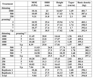
multiple range test. (The different letters at the right-upper corner represent 5% significant level) Wang et al. (2000). ...36 Table 3-2: Combination of pruning and thinning treatments ...39 Table 3-3: Means of MOE, DBH, height, taper and basic density for various thinning and

pruning treatments. (with DBH and height measurements from 2004, trees 12 years old), based on 286 trees, planted in 1992. ...45 Table 4-1: MOE of the mini bolts as measured by static compression tests and by Woodspec in

chilled condition. Values in GPa...81 Table 4-2: MOE of the mini bolts as measured by static compression tests and by Woodspec in

frozen condition. Values in GPa. ...81 Table 5-1 : Correlations (r2_{) between the ultrasound parameters and the mechanical properties}

MOE and MOR. Adapted from Sandoz et al. (2000)...87 Table 5-2: Impact of a saw cut of increased depth at midspan on the velocity, maximum peak and energy of acousto-ultrasound in a wood plank (adapted from Sandoz et al 2000)...87 Table 5-3 Velocity, based on the 1st,₂nd_{and 3}rd_{harmonic, and damping ratio (%) of the tested}

beams before artificial knots were introduced (average of 3 beams per configuration)...100 Table 5-4: Percentage of cross section and percentage of beam volume influenced by dowels of

various diameter...101 Table 5-5: Elam and E2 of a LVL-L beam with increasing number of knots drilled on the

centreline and perpendicular to individual layers as calculated from the 1st_{harmonic, from} the harmonic with the lowest value and from the average of the first 8 harmonics...115 Table 5-6: Damping ratio of a LVL-L beam with various holes drilled centred and perpendicular

to the individual layers. ...117 Table 5-7: TOF versus and resonance velocity in laminated beams ...117 Table 5-8: Comparison between the acoustic dynamic MOE and the static apparent MOE

(measured when layers are oriented perpendicular (90˚) as well as parallel (║) to the applied load). E-modulus in GPa. Static MOE not corrected for shear...120 Table 5-9: Comparison of the theoretical MOE (predicted) with the MOEs measured from

3-point-bending and acoustic testing. Values in GPa...123 Table 5-10: Impact of bifurcation on the damping ratio and the MOE. Values in brackets are

(7)

List of figures

Figure 1-1: Schematic section of a typical P. radiata stem showing new categorisation of wood

zones. (adapted from Burdon et al., 2004). --- 7

Figure 1-2: Bending stiffness according to the distance from the base of the stem and the distance from the pith. P1, P2 … refers to the numbering of boards which have been stress graded. P1 boards are centre boards while P4 boards are cut from the periphery. (adapted from Xu and Walker 2004). --- 8

Figure 2-1: Wavelength and amplitude of a compression wave ---20

Figure 2-2: Resonance pattern for the first three harmonics. The dark areas represent anti-nodes and the lighter areas nodes.---22

Figure 2-3: Mass-spring system of a log for the 1st_{harmonic as sensed by acoustics.---23}

Figure 2-4: Bandwidth of a resonant peak. ---27

Figure 2-5: The logarithmic decay in amplitude (of accelereation) of the stress wave with time of a plastic cylinder as measured by “PULSE”. ---29

Figure 2-6 Impulse response of an isolated mode displayed on a logarithmic scale.---30

Figure 3-1: Layout of the Blenheim Pruning Trail---38

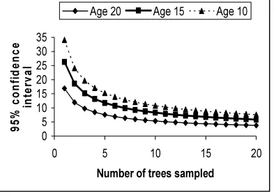
Figure 3-2: Number of measurements to be taken in order to estimate the individual side mean to various levels of precision. Confidence interval is expressed as percentage of the mean (Toulmin and Raymond 2007).---41

Figure 3-3: Number of trees to be sampled within a plot in order to estimate the plot mean to various levels of precision. Confidence interval is expressed as a percentage of the mean. (Toulmin and Raymond 2007).---42

Figure 3-4: Mean MOE of the 12 different treatments and Tukey grouping. Treatments with different letters are significantly (P < 0.05) different from each other. ---46

Figure 3-5: Mean basic density for the 12 treatments and Tukey groupings.---47

Figure 3-6: Correlation (r2_{) between MOE and basic density.---48}

Figure 3-7: Mean DBH for the 12 treatments as measured in 2004 and Tukey grouping of the 2005 measurements.---48

Figure 3-8: DBH over tree age.---49

Figure 3-9: Mean tree height for the 12 treatments as measured in 2004 and Tukey grouping of the 2004 measurments. ---50

Figure 3-10: Tree height over tree age.---51

Figure 3-11: Mean taper for the 12 treatments as measured in 2004 and Tukey grouping of the 2004 measurements.---51

Figure 3-12: Taper over tree age.---52

Figure 3-13: Mean distance from the base of the tree to the green crown of the 12 treatments as measured in 2006.---54

Figure 3-14: Mean length of green crown after the last lift (1999-2001) and in 2004.---56

Figure 4-1: Experimental steps in this study. ---64

Figure 4-2: Method for calculating the percentage of cross section occupied by a knot. ---65

Figure 4-3: Typical eucalypt bolts of the three different Groups.---67

(8)

Figure 4-5: Overlapping of branches at either end (Group 1) with the nodes and antinodes of the first 5 harmonics. The dark areas refer to antinodes for pressure (nodes for displacement).

The light areas are nodes for pressure (antinodes for displacement).---70

Figure 4-6: Overlapping of branches at midspan (Group 2) with the nodes and antinodes of the first 5 harmonics. The dark areas refer to antinodes for pressure (nodes for displacement). The light areas are nodes for pressure (antinodes for displacement).---71

Figure 4-7: Overlapping of branches at ¼ and ¾ span (Group 3) with the nodes and antinodes of the first 5 harmonics. The dark areas refer to antinodes for pressure (nodes for displacement). The light areas are nodes for pressure (antinodes for displacement).---72

Figure 4-8: MOE (%) calculated from the detectable harmonics of all eucalypt and pine samples in chilled and froze condition.---75

Figure 4-9: MOEs of the first five harmonics of group on (knots at either end). ---76

Figure 4-10: MOEs of the first five harmonics of group two (knots at midspan). ---77

Figure 4-11: MOEs of the first five harmonics of group 3 (knots at 1/4 and 3/4).---78

Figure 4-12: MOEs of the first five harmonics of resized samples. ---79

Figure 4-13: Cross section of the bolt showing the positions from where the sticks were taken.--80

Figure 5-1: Consequences of the support position using a hammer as excitation source and triangles of foam as support on the max peak of the fundamental (100%) and subsequent harmonics. ---92

Figure 5-2: Logarithmic decay curve of a 4L-4T-4L beam when exited by a hammer tap.---94

Figure 5-3: A centreline dowel drilled parallel (A) and perpendicular (B) to the individual layers of the beam. ---96

Figure 5-4: Correlation between pulse auto damping and the damping ratio based on the impulse respond method, logarithmic decrement and reverberation time---97

Figure 5-5: Velocity based on the first 3 harmonics versus percentage knot volume in a LVL-L beam with knots at midspan (size of the knot increases from left to right).--- 101

Figure 5-6: Velocity based on the first 3 harmonics versus percentage knot volume in a LVL-L beam with knots at 1/4 and 3/4. --- 102

Figure 5-7: Velocity based on the first 3 harmonics versus percentage knot volume in an LVL-L beam with 25 mm knots at various positions along span.--- 103

Figure 5-8: Influence of knots of increasing diameter at midspan on the damping ratio (solid black lines) and MOE (grey dashed lines) when drilled perpendicular to the individual layers. --- 104

Figure 5-9: 25mm edge knots drilled parallel to the layers at midspan either side of a 4L-4T-4L beam.--- 106

Figure 5-10: Influence of knots of increasing diameter at midspan on the damping ratio and MOE when drilled parallel to individual layers. --- 107

Figure 5-11: Impact of edge knots at either side at midspan drilled perpendicular the individual layers of the beams on the damping ratio and the MOE.--- 108

Figure 5-12: Impact of edge knots at either side at midspan drilled parallel the individual layers of the beams on the damping ratio. --- 109

Figure 5-13: Impact of knots of increasing diameter drilled perpendicular to the individual layers at ¼ and ¾ span on the damping ratio.--- 110 Figure 5-14: LVL beam with holes at various positions along the span. The numbers on the top

(9)

the bottom refer to the steps of the experience. Step 1 without holes. (Not drawn to scale). --- 111 Figure 5-15: LVL beam with holes at various positions along the span. The numbers on the top

mark the odd 16th_{of the span (anti-nodes for the 8}th_{harmonic) and the numbers on the} bottom refer to the steps of the experience. (Not drawn to scale). --- 112 Figure 5-16: Change in velocity of the first eight harmonics when systematically increasing the

knot volume of a LVL-L beam. --- 113 Figure 5-17: Impact of % knot volume on the damping ratio and MOE of a LVL-L beam. ---- 114 Figure 5-18: MOE of the middle layers of a LVL-L beam which are affected by increasing the

number of knots drilled centred and perpendicular to the individual layers. --- 116 Figure 5-19: Schematic setup for the 3-point bending test.--- 118 Figure 5-20: Parameters that are required for the calculation of the flexural stiffness of a

laminate (sandwiched beam) loaded perpendicular to its laminates.--- 121 Figure 5-21: Variation of the MOE and the loss factor with the number of defects in the wooden

bar. Adapted from Ouis 2000. The holes were drilled in various rows.--- 124 Figure 5-22: Anti nodes (dark areas) and nodes for pressure of the first four harmonics.--- 127 Figure 5-23: Bifurcation of the fundamental frequency of a plywood beam caused by a centreline

(10)

Acknowledgements

I wish to thank John Walker for being my supervisor and supporting me throughout the entire masters programme. Big thanks to Luis Apiolaza, my co-supervisor, especially for his advice and expertise in statistics.

The support from the staff of the school of forestry is also highly appreciated: thank you Jeanette, Vicki, David, Nigel, Lachlan, Marco and all the others.

The summer work for Forest New South Wales was a great opportunity to get some work experience, explore a new country and to make good friends. Special thanks to Carolyn Raymond for the support, assistance and advice with the study on the Blenheim Pruning Trial.

I also would like to say thank you to Roddy MacKenzie from Napier University, Edinburgh, for the cooperate research on laminated beams. Thank you for having me as a guest at your university and for showing me parts of beautiful Scotland.

Financial support from a masters scholarship granted by the University of Canterbury is highly appreciated.

Thank you to my Christchurch friends for keeping me from working too much on my thesis and for a good time in New Zealand.

(11)

Abstract

Several acoustic techniques have been used to determine elastic and damping properties of trees, logs and beams.

Time of flight (TOF) measurements in the outerwood of 14-year-old Pinus radiata

trees showed that pruning operations increased the outerwood stiffness by up to 25% compared with unpruned trees. However, at the most 5% to 10% of the increased stiffness can be explained by the fact that the outerwood of the pruned trees is free of knots, as TOF measurements are little affected by knots. Thus, it is not known what causes the increase of outerwood stiffness in the pruned trees. One possible explanation could be a smaller microfibril angle (MFA) in the S2 layer of the outerwood cells, which would cause a significant increase in stiffness. Thinning operations decreased the outerwood stiffness by up to 8%.

In small Eucalyptus nitens and Pinus radiata logs, which had branch nodes and nodal whorls at specific locations, MOE calculations (using the resonance technique) based on different harmonics gave different results. This indicates that defects do interact with acoustic waves.

Acoustic tests on laminated beams with artificial defects (holes filled with dowels) at specific locations also had a significant impact on the MOE. Moreover, it was evident that the damping ratio (evaluated from the Q- factor) of the beams increased with increasing diameter of the holes.

(12)

1 Chapter 1: General Introduction

1.1 Aim of the study

Wood is a natural material which has been used for millennia for many purposes. Today, wood is used as a raw material for a variety of products, such as furniture, structural timber in housing, wood-based panels and pulp and paper.

Wood shows large variation in its properties. The properties of wood mainly depend on its cellular, anatomical and chemical characteristics (Zobel and van Buijtenen, 1989). These properties determine the behaviour of wood during processing; moreover, they have a major impact on the features of the final product and as a consequence, the value of the wood mainly depends on its properties. Different sectors of the wood industry demand wood that has different specific requirements. Therefore it is crucial to sort or to grade wood according to its properties. Log grading systems around the world are still based on length, diameter, straightness and branch size which are all external assessments and provide almost no information about intrinsic wood properties. However, the result of such grading and sorting systems is often not sufficient, neither for forest owners, nor for the wood industry and their customers. Only with the most accurate information is it possible to achieve the greatest value recovery from the logs and to use the raw material efficiently and effectively (Xu and Walker, 2004). Therefore more consistent methods have to be used to assess wood, in particular the intrinsic properties of logs and timber. During the last decade a reasonable amount of effort has been made to develop methods and tools for the non-destructive assessment of wood properties in logs and timber and also in standing trees. One promising area is acoustics.

This thesis covers three acoustic studies:

(13)

• Chapter 4 discusses the resonance method applied to small Eucalyptus nitens

and Pinus radiata logs. Acoustics is a relatively new method to assess wood properties, and there may be uncertainties in using these recently developed acoustic tools. Branches and nodal whorls may have an impact on the acoustic behaviour of wood, although the general opinion is that acoustic waves, which roughly match with the size of the sample, are not affected by disturbances that are much smaller than their wavelength.

• Chapter 5 explores measuring various acoustic parameters in an engineered wood product which has a controlled degree of inhomogeneity. The impact of artificial defects, introduced at specific locations of the test specimens, on the elastic and damping properties is examined.

In Chapter 4 and 5 it is demonstrated that the resonance method can give different results when testing the same specimen under the same test configuration.

1.2 Wood characteristics and properties

Wood is a complex and highly ordered material. The overall performance of wood can be best described by its characteristics and properties. Often the term wood quality is used instead. When discussing wood quality one has to take into consideration that wood is used for many purposes and itself is highly variable. Different end products demand different types, or qualities, of wood. Therefore it is reasonable to describewood by its characteristics and/or properties.

(14)

trees”. A good general definition of quality has been given by Gibson (1980, cited in Zobel and van Buijtenen 1989): “quality is the totality of the attributes of a product which contributes to the satisfaction of needs”.

1.2.1 Basic characteristics

Wood structure

Wood is a complex, inhomogeneous and anisotropic material based on hierarchical structure with cellulose microfibrils and lignin as its most basic components. The proportions of the components show large variation between and within species, stand and also within a single tree. Typical composition of coniferous wood and hardwood is shown in Table 1-1.

Table 1-1: Typical composition of conifers and hardwoods (Walker, 2006)

Components Conifers Hardwoods

Cellulose 42 ± 2% 45 ± 2%

Hemicellulose 27 ± 3% 30 ± 5%

Lignin 28 ± 2% 20 ± 2%

Extractives 3 ± 2% 5 ± 3%

(15)

alignment (microfibril angle) of the microfibrils. The dominant layer is the S2 layer, in which the microfibrils are aligned at an angle of approximately 15-30˚ from the longitudinal axis of the cell. Hence, the configuration of the S2 layer plays a major role in terms of wood properties and characteristics.

The wood structure of conifers is much simpler compared with the structure of hardwoods. The wood of conifers consists of up to 95% of vertical tracheids, up to 5% horizontal ray cells and some resin canals. The more complex wood of hardwoods has short and large diameter vessel elements, tracheids, longitudinal parenchyma and it has rays with differing types of cells (Macdonald and Franklin 1969). The distribution of the vessels has a major impact on the properties of hardwoods. Within the hardwoods diffuse porous wood, where the vessels are evenly spread across one growth ring, may be distinguished from ring porous wood where the vessels are laid down almost side by side in the early wood band of each growth ring.

Density

Wood density is the oldest and most widely used criterion for the evaluation of wood. According to Bamber and Burley (1983) “it has a considerable influence on strength, machinability, conversion, acoustic properties, wearability, paper yield and properties and probably many others”.

Owing to the fact that the density of cell wall material of any wood species is almost constant (1530 kg/m3), wood density is mainly determined by the amount of cell wall material in relation to the voids. The amount of moisture in the wood has to be considered when the density is determined. Density can therefore be expressed as: green density, oven-dry density, air-dry density or basic density. The latter is a standardised method that gives a precise measure of the ratio of water saturated cell wall material to void space.

(16)

species such as Douglas fir, where the ratio between earlywood (thin-walled cells with large lumen) and latewood (thick-walled cells with small lumen) is around 1:5. In radiata pine the difference in density between earlywood and latewood is much smaller (1:1.8), which can be considered as beneficial in terms of machinability (Harris, 1981). In conifers, a reduced percentage of latewood can partly explain low density (Smith, 1980).

A study by Cown et al. (1991) on radiata pine showed that the trend for density variation within trees is that density increases radially with distance from pith and decreases vertically with increasing distance from the base of the tree.

Within the hardwoods the density contrast between earlywood and latewood is greatest in ring porous trees. In diffuse porous trees the difference is less pronounced, although the wood tissue produced early in the growing season is of lower density than the thick-walled latewood tissue.

Microfibril angle

(17)

Stiffness

Stiffness is defined as the resistance of an elastic body to deflection or deformation under an applied force. The Young’s modulus of elasticity (MOE) can be thought of as a measure of the stiffness of a material. The stiffness of a structure is of principal importance in many engineering applications. In recent years stiffness has been more frequently used to describe the mechanical properties of wood, especially the properties of structural timber (Burdon et al., 2004). The MOE of wood can be determined by static bending tests but it can also be estimated by using acoustic techniques.

Studies on radiata pine by Tsehaye (1995) and Xu (2000) revealed that stiffness varies in both the vertical (bottom to top) direction and the radial direction (pith to bark). The microfibril angle is thought to be the most important factor affecting stiffness

1.2.2 The concept of juvenile and mature wood

In a broad sense, juvenile wood is produced at a young cambial age. Thus it can be found around the pith of the stem (Barnett and Jeronimdis, 2003). Cown (1992) gave a “New Zealand” definition for juvenile wood which is “the wood within the 10 rings of the pith”. Consequently the wood outside the 10th

(18)

lignin content and shorter tracheids in gymnosperms, and tension wood with a higher cellulose content in angiosperms); a larger microfibril angle causing low stiffness and higher longitudinal shrinkage; high grain spirality; and relatively high moisture content (prior to heartwood formation) (Zobel and van Buijenten, 1989). Differences between corewood and outerwood lead to a well known radial (pith-to-bark) change of some wood properties, especially for softwoods like Pinus radiata or Pinus taeda. This is reflected by increasing stiffness, strength and stability from pith-to-bark. All of these wood properties are crucial for structural timber (Burdon et al., 2004).

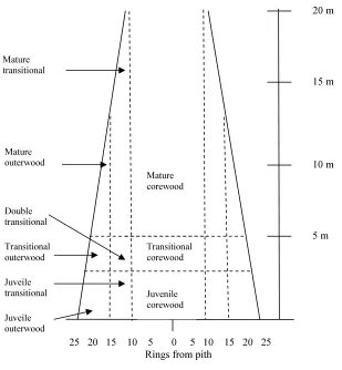
Figure 1-1: Schematic section of a typical P. radiata stem showing new categorisation of wood zones. (adapted from Burdon et al., 2004).

Burdon et al. (2004) have suggested a more accurate definition of juvenile wood, and redefined juvenile wood as “the wood near ground level of trees grown from seed, irrespective of ring number from the pith”. Moreover, Burdon et al. (2004) divided the

25 20 15 10 5 0 5 10 15 20 25 Rings from pith

Mature corewood

Juvenile corewood Transitional corewood Mature

transitional

Mature outerwood

Juveile outerwood Juveile transitional Transitional outerwood Double transitional

[image:18.595.132.441.318.652.2]

(19)

stem in a new two-way classification of wood zones (Figure 1-1). This includes a radial progression from corewood to outerwood and a vertical progression from juvenile to mature wood. The authors argue that their new classification better matches the well-established botanical concept of maturation.

A study by Xu and Walker (2004) on 62 Pinus radiata trees showed that the wood with the lowest stiffness is found in the centre of the butt log (Figure 1-2). One reason for this is probably the high microfibril angle near the base of the tree. Also a significant stiffness gradient is still evident in the first, second or third log. It also clearly reveals that the poorest quality wood is laid down in the very early or juvenile years in the life of the tree which might justify or support the new classifications made by Burdon et al. (2004).

Figure 1-2: Bending stiffness according to the distance from the base of the stem and the distance from the pith. P1, P2 … refers to the numbering of boards which have been stress graded. P1 boards are centre boards while P4 boards are cut from the periphery. (adapted from Xu and Walker 2004).

(20)

Studies of Larson (1963) and Fabris (2000) suggest that the location of the crown is an important factor which affects the quality and quantity of wood produced along the stem. It is assumed that juvenile wood is produced within the crown and mature wood below. This assumption is based on the fact that growth regulators (hormones) produced by the foliage and the apical meristem may inhibit the formation of mature wood. Thus, while those growth regulators move downwards to the base of the tree they become less effective and consequently mature wood can be produced. However, this issue is controversial and studies of Sundberg et al. (1993), Funada et al. (2001) or Savidge (2001) did not corroborate this lowered effect of plant growth regulators below the crown.

Gartner et al. (2002) tested the assumption that the bole of softwoods produces juvenile wood within the crown and mature wood below. They compared growth ring areas and widths and wood density components of the outer three growth rings in disks sampled from various vertical positions of 34-year-old Douglas-fir which had a wide range of heights from base to live crown. Gartner et al. found no statistically significant difference at p= 0.05 for any of the factors studied supporting the hypothesis that the formation of mature wood is dependent on the position of the green crown.

1.3 Pinus radiata

D.Don

1.3.1 Taxonomy and nomenclature

Pinus radiata D. Don. belongs to the subgenus Pinus (syn. Diploxylon) (‘hardpines’), section Pinus. Within that section it has recently been reassigned, along with the closely related Pinus muricata and Pinus attenuata, to a new subsection called Attenuatae van der Burgh (Price et al., 1998 and Millar, 2000). Pinus radiata

(21)

cedrosensis, var. bianta and var. radiate. Some other common names for Pinus

radiata are Monterey pine, remarkable pine and insignis pine. California pine is also a trade name.

1.3.2 General description

Pinus radiata is an evergreen tree of 20-35 m height and a DBH of 40-100 cm when growing in its natural area of distribution. These figures are highly dependent on stocking and site fertility as both play a major part in the growth pattern. However, exotic plantings can reach heights of 55 m and diameters of up to 250 cm. The wood of Pinus radiata is of low to medium density and its mechanical properties are comparable to other common softwoods, although the properties of Pinus radiata are highly influenced by factors like genetics, environment, age and silviculture.

1.3.3 Geographic Distribution

Natural Distribution

(22)

Locations of introductions

The main countries where Pinus radiata has been planted on a massive scale are New Zealand and south central Chile (approx. 1.5 million ha each). There are also considerable plantations in southern Australia (> 700.000 ha) and northern Spain (approximately 220000 ha). Other significant plantations have been established in South Africa, Ecuador Argentina and Italy. This comes to a total ex situ plantation area of more than 4 million ha, which is more than 99.7 % of the global estate (Lavery and Mead, 1998).

1.4 Eucalyptus nitens

Maiden

1.4.1 Taxonomy and nomenclature

Eucalyptus is a diverse genus of trees within the plant family Myrtaceae. A new formal classification of the genus Eucalyptus was recently developed by Brooker (2000). It includes 13 subgenera in the concept of the whole genus Eucalyptus, six of them consisting of only a single species. Within the 13 subgenera are more than 700 species, most of them native to Australia. Only a few species are found in adjacent parts of New Guinea and Indonesia and one as far north as the Philippines. Eucalyptus nitens belongs to the distinctive group of eucalypts that are characterised by very remarkable, large, sessile, glaucous juvenile leaves to the tall sapling stage, seen most prominently in E. globulus (Brooker, 2000). Some other common names for

Eucalyptus nitens are shining gum and silvertop.

(23)

Eucalyptus nitens is a fast growing hardwood tree that can grow to a height of 70 m. The bark of Eucalyptus nitens is smooth throughout or has a thin zone of rough grey bark in the basal metre of the trunk. Further up the trunk the predominantly smooth bark is pale grey to greenish-grey but with patches of white, cream or pale brown with some horizontal black scars. The usually straight grained wood of Eucalyptus nitens

has an air-dry density of approximately 700 kg/m3

. The medium textured heartwood is of straw colour with pink or yellow tints (Bootle, 2005). The wood is used for general building construction, flooring, joinery, panelling, furniture and pulp.

1.4.3 Geographic Distribution

(24)

(25)

2 Chapter 2: Introduction on Acoustics

Acoustics can be used for non-destructive testing of wood. Ross and Pellerin (1994) state, that “nondestructive materials evaluation is the science of identifying physical and mechanical properties of material without altering its end-use capabilities”. Acoustic techniques can be applied to get a fast estimation of the elastic and damping properties of wood. The material’s elasticity can be described by the relation between stress and strain. In the elastic range (the linear region between stress and strain) Hooke’s law relates stress and strain by the means of the MOE:

ε σ ₌_E where;

σ= stress, E= Modulus of elasticity and ε= strain.

Damping reduces the amplitude of oscillations in an oscillatory system by dissipating vibration energy into heat. Damping is often characterised by the loss factor which is defined as the ratio of lost energy to the vibratory reversible energy during one cycle of vibration (Ouis, 2002).

The dynamic properties of solid materials are often frequency- and temperature- dependent. Unlike many other solid materials, the damping and elasticity properties of wood become frequency-dependent at a few kHz. It was found that the dynamic MOE tends to increase with frequency. Ferry (1980) reports that the curve of frequency variation of the MOE of organic polymers passes a turning point at about the same frequency as when the loss factor goes through a maximum. Thus, it can be assumed that elastic and damping properties are dependent on each other (Ouis, 2002).

Areas where acoustics can be applied are:

• Defect assessment in sorting and grading of wood and timber

• In-place assessment of wooden members

(26)

2.1 Wave propagation in wood

Wood is regarded as an orthotropic solid having three mutually perpendicular planes of elastic symmetry: longitudinal, radial and tangential (Bucur, 1996). Consequently the propagation of sound in wood is much more complex than in isotopic materials. Wave propagation in isotropic materials should be considered first. Longitudinal waves, where particle motion is along the propagation direction can be distinguished from shear waves or transverse waves where the particles vibrate perpendicularly to the propagation direction. However, in wood, longitudinal and transverse waves can also travel out of their principal symmetry direction. Surface waves, which can propagate in any direction, are found in isotropic and anisotropic materials.

The mathematics for anisotropic material like wood are more complex than those of isotropic materials. Nevertheless, it is possible to apply acoustics in anisotropic materials. There are considerable differences in propagation speed of acoustic waves along these directions; for example, the velocity in the longitudinal direction is five times greater than in the radial direction (Harris and Andrews, 1999).

To meet the requirement of homogeneity, the wavelength must have a greater magnitude than the inhomogeneity of the sample (Feeney et al. 1996).

2.2 Acoustics used to determine the elastic properties of wood

(27)

same mechanisms that determine the static behaviour of such material” (Ross and Pellerin, 1994).

The most common way to introduce acoustic waves into logs or lumber is a light tap with a hammer. To generate compression waves that travel along the length of the specimen, one of the cut ends of the specimen has to be excited. From the point of impact the waves start to spread out into the specimen and only two propagation speeds are evident: the dilatational speed of compression and the shear speed of distortions. There are multiple interferences and reflections of these two wave types within the boundary conditions of the sample; however, after the travelling signal has passed a certain distance it can be identified as a plane wave if the lateral dimensions of the rod are small in comparison to its length (Andrews, 2002). The way a sound wave (stress wave) propagates through a body is correlated with the body’s intrinsic properties. By measuring the velocity of the travelling wave and by using the one-dimensional wave equation:

δ

× = =_E _V2 MOE

it is possible to calculate the dynamic MOE where;

MOE or E (Pa) stands for the Modulus of Elasticity, V (m/s) for velocity and δ

(kg/m³) for the density of the wood.

(28)

2.3 Factors affecting stress wave-transit time in timber

According to Gerhards (1982), who summarized the results of previous studies in this area, as a rough approximation, the propagation speed of stress waves decreases by 1% when the moisture content increases by 1% within the hygroscopic range. Further, a rise in temperature by 1˚ Fahrenheit (between 0 and 200˚ Fahrenheit) causes a drop in the propagation speed of approximately 0.05% for timber at moisture content of 12%. This temperature dependence of stress wave velocity in timber is also affected by the moisture content. With increasing moisture content the influence of temperature on the stress wave velocity becomes stronger.

As summarised by Gerhards (1982), various studies showed that the grain angle has a major impact on the velocity of stress waves. Sound travels along the grain about three times faster than perpendicularly to the grain. The velocity decrease is most pronounced within the first 30˚ from the longitudinal direction (probably following Hankinson’s formula).

(29)

2.4 Acoustic methods

Wood can support a variety of wave types and because of the fact that waves can only reveal things that are comparable to their wavelength, it is important to generate the right wavelength when looking at particular properties (Bucur, 1996). Many methods using different wavelengths have been studied and are used on standing trees, logs and wood products to measure elastic properties or to reveal defects. The most common are: the stress wave technique, Acoustic Emission (AE), Acoustic Ultrasonic (AU), Ultrasonic Techniques and Acoustic Microscopy (Buccur, 1996).

The common opinion is that high frequency waves have to be used to detect defects like knots or resin pockets. So-called Ultrasonic techniques use vibrations similar to sound waves but at much higher frequencies (> 20 kHz) (de Oliveira et al., 2002). A major problem of ultrasonic waves in wood is that they are strongly absorbed in green wood. However, this problem is less evident in dry wood.

In this study, the stress wave technique, operating with relatively low frequencies (audio range), is used to calculate the elastic properties (MOE) of young Eucalyptus nitens and Pinus radiata trees and the elastic and damping properties of laminated beams. There are basically two distinct acoustic methods that can be applied to assess the MOE: the time of flight (TOF) and the resonance method.

2.4.1 Time of flight method

(30)

results. The TOF method has been applied to standing trees, logs, timber and wood-based panels.

2.4.2 Resonance method

The resonance method can only be applied when the sample has two cut ends, thus it is not suitable for measuring MOE in standing trees. A stress wave is introduced at one end of the sample from where it travels forwards and backwards between the two cut faces of the log introducing standing waves. The signal is usually picked up from the other end of the sample using a microphone or an accelerometer.

The resonance method provides more information and also gives more reliable results than the TOF method, which is mainly due to the fact that the velocity of the wave is calculated on up to several hundred passes through the sample (Grabianowski, 2003). Resonance methods produce standing wave patterns called harmonics or modes, which match the size of the sample.

Standing waves are formed as the result of the perfectly timed interference of two waves passing through the same medium (Kane and Sternheim, 1988). A standing wave pattern is not actually a wave; rather it is the pattern resulting from the presence of two waves (sometimes more) of the same frequency moving in opposite directions within the same medium. This study focuses on compression waves, thus they are discussed in more detail than, for example, bending waves.

(31)

Figure 2-1: Wavelength and amplitude of a compression wave

A blow by a hammer at one end of a specimen (log or beam in this study) will force the particles close to the impact to move in the direction of the impact. As a consequence, the adjacent particles are also pushed in that direction, creating an area of high compression which proceeds to pass through the specimen. Meanwhile, the particles at the impact end will vibrate back. It is the elasticity of the medium which controls the return of the displaced particle towards its equilibrium position. Due to the inertia of the particle the particle will pass its equilibrium position and thereby pulling particles apart, creating a low pressure region. This low pressure area then follows the high pressure area. Thus, a compression wave, where particles are pushed back and forward parallel to the direction of the transmitted energy, consists of areas of high compression and areas of low compression (rarefactions). When the wave front hits the other end of the specimen it is reflected and starts to interfere with the waves coming from the opposite direction. If it now happens that the compression of one wave meets up with the compression of a second wave, the pressure at that particular location will be even greater. Such a scenario is called constructive interference. Constructive interference also occurs when two low pressure areas travelling in opposite directions meet and thereby create an area of even lower pressure. Locations where constructive interference continually occurs are known as antinodes. Antinodes are therefore locations where the specimen undergoes maximum positive and negative change in pressure.

(32)

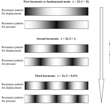
takes place will not be pressurized, as the tendency of compression to push particles together is cancelled out by the tendency of rarefaction to pull particles apart. If destructive interference continually occurs at the same location, then this region will form a node. A standing wave pattern always consists of an alternating pattern of nodes and antinodes. However, once a medium starts to vibrate, different standing wave patterns, called harmonics, can be obtained (Halliday, Resnick and Walker, 1997). The wave pattern with the longest wavelength that fits into a medium (in this study, a log or a beam) is referred to as the fundamental mode and has a wavelength of twice the log length. The next possible pattern, called second harmonic or first overtone, which fits inside the log has a wavelength that is equal to the log length. The distribution of the nodes and antinodes along the specimen is of great interest.

The distribution of pressure and displacement within the specimen

(33)

[image:33.595.87.461.124.484.2]

Figure 2-2: Resonance pattern for the first three harmonics. The dark areas represent anti-nodes and the lighter areas nodes.

The wavelength of the nth harmonic can be calculated by the equation:

λn = 2 L/n

and the corresponding frequencies are found from:

fn = (n/2L) × V

where;

V = velocity, f = frequency, λ = wavelength and L= (log) length

Resonance pattern for pressure

First harmonic or fundamental mode. λ = 2L/1 = 2L

Second harmonic. λ = 2L/2 = L

Third harmonic. λ = 2L/3 = 0.67L

Resonance pattern for pressure Resonance pattern for displacement

H

igh

er f

req

uen

cie

s

Resonance pattern for displacement

(34)

A vibrating log in which compression waves are travelling forth and back can be described by a set of masses and springs. The positions where the log has antinodes for displacement refer to a mass. The masses are connected with springs (Figure 2-3).

Figure 2-3: Mass-spring system of a log for the 1st

harmonic as sensed by acoustics.

Applying Hooke’s law and using the definition of Young’s modulus with the definitions of stress σ = Force/Area and strain ε= ∆l/l, this becomes:

l l E A

F _∆

=

Therefore, in tension or compression the force on an object is proportional to its elongation:

l k F ₌ _∆

where k is the spring constant which is defined by:

l EA

k₌

From the definition of k it follows that the spring constant can be changed by altering the cross-sectional area. An increase of the cross-sectional area will increase the spring constant.

2.4.3 TOF method versus resonance method

Andrews (2002) compared acoustic speeds measured by the TOF and the resonance method. Observations in the past have shown that there is some discrepancy between both methods, especially in short samples. Once a wave is introduced into an elastic material only two propagation speeds can be found: the dilatational speed of compression and the shear speed of distortions. Andrews’ (2002) examinations

Mass-spring system for first harmonic

(35)

showed that there is a provable difference in velocity between the TOF and the resonance method when measuring the same logs. The TOF speed was significantly higher (approximately 1.25 times) than the resonance speed. The time that is needed to travel through the log (during a single pass) was calculated based on the multi pass resonance method. Looking only at the first pass between both ends, Andrews observed that there was a small amount of energy which was arriving earlier and thereby stopping the time measurement. However, the explanation for this is that some energy travels faster than the main wave front. This weak signal, called incremental speed, travels in a straight line from one end to the other end of the sample without being reflected from the edges of the sample (Andrews, 2002). However, this faster travelling energy dies away inversely with distance squared and the measurable wave becomes a plane front. This is the reason why this phenomenon can be ignored when acoustic velocity is measured by resonance methods.

To obtain the right data from TOF tools, it is crucial to distinguish between the fast incremental and the slower propagation speed of the developing plane wave. Thus, the sensitivity and the setting of the detecting probes have a major impact on the performance of the tool. The influence of the incremental speed is highest in short samples. The reason is twofold: as already mentioned, the incremental speed dies away inversely with distance squared; and secondly the time difference between the incremental speed and the “main” wave is relatively higher over short distances. According to Andrews, the consequences of this are that acoustic velocities based on TOF measurements are often overestimated by a factor up to 1.3, especially in relatively short samples with a high diameter to length ratio. The following equation can be used to avoid an overestimation of the MOE when measuring very short samples:

δ

2

3 . 1 _

   

= V

(36)

When the length is about ten times the diameter, it can be assumed that the correction factor can be neglected. However, Andrews (2002), advocates further research to verify this length to diameter ratio.

2.5 Damping properties of wood

Damping is evident in all real systems. Even in systems with small damping the system will still oscillate and the amplitude of the vibration will decay exponentially with time. In an over-damped system, no vibration will be found and after excitation the mass will return slowly to its original position. If a system is critically damped it just fails to oscillate and returns to its original time in the fastest possible time: for example, suspension systems of vehicles should be critically damped. The damping ratio compares the damping constant of the system with the critically damped case, and thereby expresses the viscous damping of the system (Smith, Peters and Owen, 1996). The damping ratio (often expressed as a percentage) for lightly damped systems is approximately half the loss factor.

There are three main factors that affect the damping properties of wood: the geometry of the sample and the material characteristics of scattering and absorption. Scattering and absorption are highly dependent on frequency, anisotropic direction and wood species (Buccur, 2005).

2.5.1 Methods to calculate damping

There are many different methods that can be applied to calculate damping. They can be divided into three groups:

• Vibration decay measurements (time domain)

• Bandwidth determination of measured modal resonances (frequency domain)

(37)

This study does not deal with the steady-state technique which is based on the energy balance of vibrationally excited structures.

The complete dynamic behaviour of a structure can be described by its individual modes (harmonics) of vibration. The so-called modal parameters characterize the modes in a given frequency range (Brüel & Kjær, 1994). The modal parameters are:

• The resonance or modal frequency

• The damping of the resonance – the modal damping

• The mode shape

Damping can be described by many factors which are all interrelated; for example, loss factor, damping ratio, quality factor, reverberation time and logarithmic decrement.

Quality Factor method

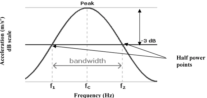
The quality factor or Q factor is an indicator of the "quality" of a resonant system. Resonant systems respond to frequencies which are close to their natural frequency much more strongly than they respond to other frequencies. The Q factor measures the sharpness of the resonance peak, as displayed in a frequency response function (FRF) spectrum or by fast fourier transform (FFT), and therefore this method belongs to the frequency domain category. Systems with a high Q factor resonate with greater amplitude at the resonant frequency compared with systems with a low Q factor. Damping within the system decreases the Q factor.

The Q factor is defined as the resonant frequency (frequency of the peak) f0 or fc

(38)

ratio 10 which takes account of the fact that the perception of loudness of the human ear is roughly logarithmic.

The Q factor can be calculated by the following equation:

f f f f f

Q c c

∆ = − =

1 2

where;

Q = Q factor, f2 = the upper, f1 = lower half-power frequency, ∆f = f2 - f1 and fc =

frequency of the peak

The Q factor is related to the damping ratio by the following equation:

Q

2 1 =

ξ

where;

[image:38.595.136.481.495.659.2]

Q = Q factor and ξ= damping ratio

Figure 2-4: Bandwidth of a resonant peak.

The accuracy of the frequency measurements is determined by the frequency resolution of the measurement. The accuracy can be increased by reducing the

Frequency (Hz)

Ac

ce

ler

at

ion

(m

/s

2 )

dB

sc

al

e

(39)

frequency range of the baseband, or making a zoom measurement around the frequency range of interest.

Whenever the Q factor was used in this study, it was given by the auto damping function of the “PULSE” unit which is based on the fundamental frequency. This automated function is very useful especially in terms of time efficiency. However, it is also possible to calculate the Q factor on subsequent harmonics. In this study calculating the damping based on the fundamental frequency was chosen. The reason for this is twofold. Firstly the fundamental frequency is usually the strongest mode in the FRF spectrum and secondly, higher frequencies receive higher damping which might affect the accuracy of the frequency measurement of subsequent harmonics.

Logarithmic Decrement

The logarithmic decrement provides a variable which tells how quickly the motion decays. It therefore belongs to the time domain measurements. It is important to point out that the logarithmic decay curve displays the whole frequency spectrum; therefore logarithmic decrement measurements give accurate results when only one resonance is present (Brüel & Kjær, 1994). Figure 2-5 shows a typical decay curve (of a homogeneous cylinder of plastic) where the time is plotted against acceleration. Logarithmic decrement can be calculated by the following equation:

n

e

_X

X

n

log

1

1 =

δ

where;

δ = logarithmic decrement and X1 and Xn are two amplitudes n cycles apart.

Logarithmic decrement is related to the damping ratio (ξ) by the following relationship:

π

δ

(40)

[image:40.595.97.496.114.326.2]

Figure 2-5: The logarithmic decay in amplitude (of accelereation) of the stress wave with time of a plastic cylinder as measured by “PULSE”.

Impulse Response method

The impulse response method in its simplest form is used by woodmen to judge the quality of a tree trunk by ear. When the trunk is hit with a hammer (impulse) the vibrational response is detectable by the human ear owing to the low resonance frequencies of a log (< 20 kHz).

(41)

[image:41.595.134.461.122.324.2]

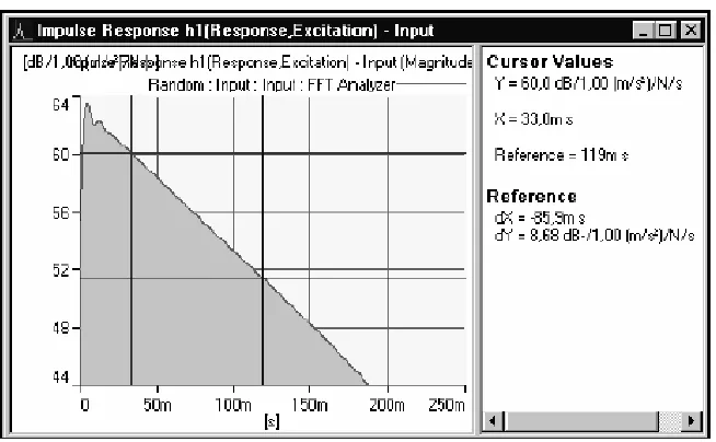
Figure 2-6 Impulse response of an isolated mode displayed on a logarithmic scale.

The decay rate σ _{for the isolated mode is related to the time constant} τ _by

(Brüel&Kjær, 1999):

σ τ ₌ 1

The decay corresponding to time constant τis given by the factor e–1, or in dB:

-20loge= –8.7 dB.

The damping ratio ξ is related to the decay rate by:

f f τ π π

σ ξ

2 1

2 =

=

Reverberation Time method

(42)

decay and knots in logs and timber. The reverberation time T60 is the time that is required for the energy of the system to drop to one millionth of its initial value, or alternatively, the time within 60dB decay in energy or amplitude can be observed. The following equation can be used to calculate the loss factor based on reverberation time (Cremer and Heckl, 1988):

60 60

6 ₂_.₂

2 10 ln

fT

fT ≈

= π

η

2.6 Acoustic tools used in this study

2.6.1 The TreeTap time of flight tool

(43)

2.6.2 The WoodSpec resonance Tool

Woodspec was designed and build by Industrial Research Ltd. The WoodSpec tool consists of a flexible pc-based data acquisition and spectral analysis package which provides a graphic presentation of the time trace and its spectral analysis. The acoustic signal reverberates within the sample and from the frequency of the reverberation the acoustic velocity is determined using the following relationship:

V = 2 × l × f

where;

V stands for velocity, f for frequency and l for (log) length.

It is possible to run WoodSpec in three different modes: trigger, sweep and monitor. The trigger mode can be either used with a microphone or an accelerometer to pick up the acoustic vibrations from one end of the sample. The acoustic vibrations are launched into the sample by hitting the other end with a ball bearing on a string. The display of the trigger mode shows the amplitude of the signal with time (decay curve), and in a second window the peaks of the acoustic spectrum, which refer to subsequent harmonics, are displayed. In a third window the velocity of the acoustic signal is shown. Moreover, the frequencies of the first harmonic (fundamental mode) and detectable subsequent harmonics (overtones) are displayed. A detune factor, based on the first harmonic (fundamental mode), is calculated for subsequent harmonics. In an isotropic material the frequency of the nth

(44)

2.6.3 The “Pulse” multi channel analyser

The “PULSE” multi-channel analyser platform, developed and distributed by Bruel and Kjær (B&K, UK), is a windows PC-based tool that uses up to nine signal channels to perform simultaneous sound-level or acceleration measurements. By using an endevco 8202 model hammer and 3608-B TEDS cubic uniaxial accelerometers (also by B&K ), the transducers used and the calibration history are recorded automatically by the PULSE. These accelerometers have a reccomended upper limit of 8 kHz. These signals are then subject to a variety of real-time analytical applications, including time response, impulse response, Fast Fourier Transform (0% overlap, 4600 lines), automated damping ratio and reverberation time calculations, and up to 1/24 octave Constant Percentage Bandwidth analysis. This allows for imediate validation of the test. It facilitates a singal generator, including fixed and swept sine or dual sine waves and random pink or white noise generation. The “PULSE” has a maximum frequency limit of 26.6 kHz. Features include the ability to cross-reference signals from the impact energy and the response from the accelerometers, multipe trigger settings and a recording facility.

2.6.4 The Pundit tester

(45)

(46)

3 Chapter 3: The Impact of pruning and thinning on young

Pinus radiata

_trees

3.1 Introduction

The acoustic properties of 14-year-old Pinus radiata trees, growing in 12 plots (two replicates) which had been treated differently in terms of pruning and thinning, were measured to investigate whether there is any correlation between acoustic velocity in the outerwood and the pruning schedule and different thinning treatments. The impact of pruning and thinning on the basic density, DBH, tree height and taper was also examined.

3.2 Literature review

Wang et al. (2000) investigated the effects of thinning and pruning in a 20-year-old Taiwania (Taiwania cryptoerioide) trial on wood quality using an ultrasonic wave method (SYLVATESTTM

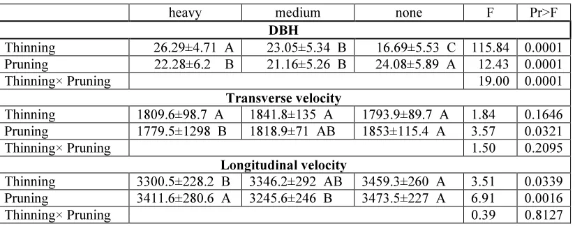
). In their study thinning, pruning and their interaction had a significant impact on DBH and (Table 3-1). They found that a heavy thinning treatment with no pruning increased DBH growth and non-thinning with heavy pruning inhibited DBH growth. Also the longitudinal velocity was significantly influenced by thinning and pruning and the longitudinal velocity in unthinned treatments was significantly greater compared to heavy thinning treatments.

(47)

[image:47.595.94.506.141.303.2]

Table 3-1: ANOVA table of DBH, transverse velocity, and longitudinal velocity by Duncan’s multiple range test. (The different letters at the right-upper corner represent 5% significant level) Wang et al. (2000).

In a more recent study on the same plantation Wang et al. (2005) repeated the acoustic measurements after trees were harvested (tree age approximately 22 years) and also did mechanical bending tests to verify the results from acoustic testing. This time measurements were on air-dried beams (2.2 m long and a cross-section of 8.9×3.8 cm) and air-dried small clear specimens (24×1.5×1.5cm) cut from approximately breast height position.

Wang et al. (2005) found that higher values for dynamic MOE, static MOE and MOR were obtained in the following order: unthinned > medium thinning > heavy thinning. The trend for the pruning treatments was: medium pruning > no pruning > heavy pruning. However, not all results were statistically significantly different. For example, both the dynamic MOE and the static MOE revealed a significant (P < 0.05) difference between the heavy-thinned and the unthinned treatments. It is also interesting to note that the dynamic MOE was approximately 20% higher than the static MOE (the same observations were made in Chapter 4 of this study). Both studies by Wang et al. (2000 and 2005) concluded that better average qualities of lumber can be obtained from unthinned stands that have received a medium pruning treatment (3.6 m from the root base upward).

Cown (1973) examined 10-year-old radiata pine trees which had undergone severe silvicultural treatments. Of interest were growth rates and intrinsic wood properties.

heavy medium none F Pr>F DBH

Thinning 26.29±4.71 A 23.05±5.34 B 16.69±5.53 C 115.84 0.0001 Pruning 22.28±6.2 B 21.16±5.26 B 24.08±5.89 A 12.43 0.0001

Thinning× Pruning 19.00 0.0001

Transverse velocity

Thinning 1809.6±98.7 A 1841.8±135 A 1793.9±89.7 A 1.84 0.1646 Pruning 1779.5±1298 B 1818.9±71 AB 1853±115.4 A 3.57 0.0321

Thinning× Pruning 1.50 0.2095

Longitudinal velocity

Thinning 3300.5±228.2 B 3346.2±292 AB 3459.3±260 A 3.51 0.0339 Pruning 3411.6±280.6 A 3245.6±246 B 3473.5±227 A 6.91 0.0016

(48)

Cown reported that stem diameter growth was reduced by pruning treatments, but only for a short period after treatment. Moreover, pruning increased the mean wood density by up to 7%, but this effect also tapered off after 2-3 years. The only significant change in intrinsic wood properties was a reduction in tracheid length caused by thinning.

Pape (1999) reported that thinning reduced the juvenile wood content in stands of Norway spruce (Picea abies). Zobel and van Buijtenen (1989) also pointed out that thinning generally decreases the juvenile wood content.

Lasserre et al. (2004) investigated the influence of initial stand density and genetic population on corewood dynamic stiffness of 11-year-old Pinus radiata. They found a significant impact of planting density (P < 0.001) and genetic population (P < 0.01) on stiffness. Plots with high initial stocking showed an MOE that was on average 1.7 GPa or 34% higher than plots with low initial stocking. The DBH was negatively related to MOE (P < 0.01). However the interaction of planting density and genetic population had no significant impact on stiffness. When DBH was introduced to the model as a covariance, the variation in stiffness and genetic population was reduced but still significant. According to Lasserre et al. (2004), initial stocking is a very important factor in terms of stiffness. It is of interest, that initial stocking and genetic population independently affect stiffness.

3.3 Location and site-characteristics of the Blenheim Pruning Trial

The study material came from Blenheim State Forest No 993, also known as the Blenheim Pruning Trial in the Macquarie region of New South Wales, Australia. The trees were planted in 1992 and the plots were established in November 1996. In December 1996, the plots were non-commercially thinned to 1000 stems/ha.

(49)

the months with maximum rainfall are June–August (average 75 mm) (Kovac et al. 1990). The average temperature in this region is 12˚C, with the warmest months in January and February (average 17˚C) and the coldest months in June–August (average 4˚C).

The Blenheim Pruning Trail lies in the Oberon landscape, which covers an extensive area of undulating to rolling low hills with elevations ranging from 980- 1336 m and slopes from 6-20%. Red earths are the dominant soil type especially on the mid to upper slopes. The geological unit is the Rockley Volcanics and Triangle Group. The parent rock code consists of andesite, tuff, grey slate, quartz and feldspathic greywacke. The topsoil of a typical red earth can be described as a dark-reddish brown, fine-sandy loam with weak structure and a pH of 6.0 at a depth of 20 cm. The subsoil gradually changes to dark-reddish brown, sandy clay loam with weak to moderate structure and a pH of 6.0.

3.3.1 Layout of the Pruning Trial

The trail is divided into 12 plots, all of which have been treated differently in terms of pruning and thinning (Table 3-2). The trial consists of two replicates (Figure 3-1).

Figure 3-1: Layout of the Blenheim Pruning Trail

Replicate 2 Plots 17-24 Plots 14-16 Plot 13 Replicate 1

(50)

The trees of the rectangular-shaped plots were planted in rows running east to west. The initial stocking of the plots in replicate 1 was approximately 1000 stems/ha. The initial stocking of the plots in replicate 2 was approximately 1400 stems/ha. The difference between the replicates is due to the fact that cuttings were used in replicate 1 while seedlings were used for replicate 2. When the trees were planted it was not intended to use them for a trial study. The trial was established in 1996. At this time the plots of replicate 2 were thinned to 1000 stems/ha. The plots are aligned in a north to south direction. The plot size for the 1000 and 500 trees/ha thinning treatment plots is 0.126 ha. They are spread over 21 rows with six trees in a row. The actual measurement plot consists of 30 trees, which are surrounded by at least two rows of buffer trees (belonging to the same plot) to avoid undesirable interaction with the treatment of adjacent plots. The plot size of the 250 trees/ha thinning treatment plots is 0.186 ha, with 31 rows of six trees. These plots consist of 13 measurement trees only. The combination of treatments of the 24 plots are summarized in

Table 3-2.

Table 3-2: Combination of pruning and thinning treatments

Plot 7 in replicate 1 and plot 24 in replicate 2 were treated as control plots since they did not receive any treatment after they had been thinned to 1000 trees/ha in 1996. It has to be emphasised that this trial is not a spacing trial. When the plots were thinned, trees of abnormal growth form, such as double leaders, broken tops or butt sweep, were preferably cut out, and those trees showing good form retained.

Pruning Treatments Thinning

Treatments Unpruned 3m green crown _remaining 5m green crown _remaining 7m green crown _remaining 1000 Stems/ha _{(Treatment A/Up)}1000 Stems/ha _{(Treatment A/3)}1000 Stems/ha _{(Treatment A/5)}1000 Stems/ha _{(Treatment A/7)}1000 Stems/ha

(51)

In this trial, the distance between the base of the tree and the green crown was not the criterion for the pruning schedule. The green crown starts where a whorl has at least three live branches. The crucial criterion was the length of the green crown that remained after pruning. Thus, the plots had to have a certain average tree height before pruning was possible. The pruning treatment was started in 1997 when the trees were five years old. The plots with the 7 m green crown were pruned in the following year because the tree height was only around 7 m in 1997. The plots were thinned at the same time as when they received their first lift, which was between 1996 and 1998. The unpruned plots (excluding the control plots) were thinned in 1997. The plots received a second and a third lift to readjust the length of the green crown to either three, five or seven metres. The maximum delay between the 1st

and the 3rd

lift was three years. Thus the last plots received the final lift in 2001.

3.4 Methodology

3.4.1 Sampling strategy

Toulmin and Raymond (2007) developed a sampling strategy for measuring acoustic velocity in standing radiata pine using the TreeTap time of flight tool. They over sampled the variables of interest to determine the sample size required to estimate the mean of one side, tree, plot and stand to a level of precision with a 95% confidence interval. The variance component (σ2_{) was used to determine the sample size required}

(n) to estimate the mean of the side, tree, plot, and stand to a required level of precision (± L) with a 95% confidence interval (which is a common level in applied science), using the equation (Snedecor and Cochran, 1967):

2 2_/

4 L

n₌ σ

Acoustic Studies on Wood