An Adaptive Computer Based System for the Prescription of Warfarin

(1)

An Adaptive Computer-Based System for the

Prescription of Warfarin

Mark Mayo

Department of Computer Science

University of Canterbury

Christchurch, New Zealand

(2)

(3)

Abstract

(4)

(5)

Introduction

“The intellect has little to do on the road to discovery. There comes a leap in consciousness, call it intuition or what you will, and the solution comes to you and you don’t know how or why.”

–Albert Einstein

Drug prediction has long been an interesting and yet frustrating area of research in the medical field. The variations in patient metabolism, the interactions between medication and a number of other external effects cause many difficulties for the accurate prediction of the effects of, and thus prescription, of medi-cation. All of these difficulties are experienced when trying to predict warfarin, which is primarily used as an anticoagulant in patients with artificial heart valves, to maintain a consistent thickness of the blood.

The administration and prescription of warfarin has long been difficult to manage — primarily due to inexperience, over-cautiousness, and often guesswork. Patients can differ enormously in their require-ments, based not only on their need for warfarin, but also on the varying quantities necessary to counteract differences in metabolism, weight and other affecting factors (Breckenridge 1977).

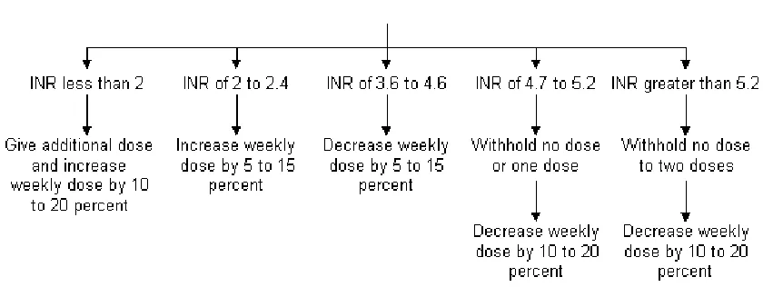
Currently, the blood thickness levels of patients on warfarin are tested every few weeks, or even days. Their results are sent to their cardiologist or their family doctor, who uses a set of guidelines or ad-hoc approach in an attempt to accurately prescribe the drug, aiming to maintain a target range for their blood reading. Inaccurate prediction of the effects and therefore prescription of the drug can cause a number of undesirable consequences, potentially resulting in clotting on the patient’s valve if the blood becomes too thick, or alternatively, thinning the blood too much, resulting in serious haemorrhaging.

These guidelines or approaches currently used are often inadequate for many patients, and can often lead to incorrect or at best inaccurate predictions of patients’ warfarin requirements. A method is required that involves a unique, dynamic model for each patient, accommodating the differences between patients, as well as taking into account the external factors that contribute to their requirements.

Since the first use of computers in the 1940s to decode messages, machines have become more power-ful and, with correct programming, are able to mimic many of the learning processes demonstrated by humans. Machine learning has become a large area of interest in Computer Science, in character or speech recognition, design engineering and object classification. As machine learning techniques have begun to be used successfully in many areas where humans currently fail (see Chapter 3), or are being used to improve on human performance, the prediction of warfarin presents itself as an area where machine learning may be of invaluable assistance.

(8)

7

thickness of the blood.

The aim of this report was to demonstrate a series of simple machine learning approaches to warfarin prediction. First, we show how the systems can learn to “mimic” an expert’s style or method of prescrib-ing warfarin dosages, based on the patient’s history of INR readprescrib-ings and the resultant prescribed dosages. Secondly, we show that the systems can accurately predict patient INRs, based on recent dosages given to them, and their INR history. This task is significantly harder than the first, requiring more accuracy as the algorithms cannot simply mimic the current expert, but instead must learn to formulate a method of prediction for the INR readings.

In cCapter 2, we present previous work in relation to the prescription of drugs, especially that of war-farin. We also look at current computer-based medical prescription systems, and evaluate their advantages and disadvantages. Finally, we examine a few potential machine learning techniques that may be applied in order to prescribe the correct dosage of warfarin, and predict the patient’s INR based on the dosage administered to that patient.

(9)

Chapter 2

Background

2.1 Warfarin

In 1924, Schofield noted a haemorrhagic disorder in cattle that appeared to result from the ingestion of rot-ten clover. Roderick, however, traced the cause of the bleeding disorder to a reduction in plasma prothrom-bin, and in 1939, Campbell and Link identified the hemorrhagic agent as bis-hydroxycoumarin (dicumarol) (Lodwick 2002). Because the first use of the compound (which came to be known as WARFARIN, based on the acronym for the patent holder, Wisconsin Alumni Research Foundation), was as a rodenticide, therapeutic applications were not initially recognised. Further research indicated that the drug could be counteracted with vitamin K. However, dosage administration was mostly still an unresearched area. Doc-tors were becoming aware of the potential benefits of warfarin, realising that thinning of the blood could avoid clotting and help patients with damaged blood vessels — where the thinner blood could help the heart pump properly.

Coumadinˆa (warfarin) was given to President Eisenhower when he had a heart attack in 1956. Since then it has become one of the most widely prescribed drugs in the world.

Warfarin therapy requires that coagulation parameters be assessed approximately every few weeks, and changes in dosages are determined by cardiologists, or even general practitioners. Doctors are often inex-perienced in anticoagulation prediction and, in addition, the task is routinely assigned to junior doctors or assistants. In the study by Doble & Baron (1987), an analysis of anticoagulation control of warfarin by junior hospital doctors, found that only 47% of the blood results were within the previously recommended therapeutic range.

Appropriate dosage requirements of warfarin, however, remain frustratingly difficult to predict, even for the experienced. International Normalised Ratio (INR) readings of the level of anticoagulation are prone to fluctuation (Routledge 1977), and careful monitoring is required in order to prevent either bleeding or clotting of the patient’s blood. The monitoring process is costly in terms of both medical and administra-tive staff time, and is often subject to varying degrees of guesswork. In fact, previous reports of outpatient anticoagulation practices have found that patients are only adequately anticoagulated 50% to 85% of the time (Duxbury 1982), (Copplestone & Roath 1984).

(10)

2.2 Near-patient testing devices 9

second group were “disappointing”. The conclusion of the paper was that the standard of long-term antico-agulant treatment should be improved by continuous review of control and by “therapeutic quality control.”

To complicate matters, in addition to a patient’s warfarin requirements being prone to fluctuation, the effect of a dosage change is usually noticeable only after a few days, due to the long effective half-life of the drug (around 36-48 hours) (O’Reilly 1968), making it difficult to judge the effectiveness of recent changes in patient dosages.

2.2 Near-patient testing devices

As doctors are increasingly burdened with work and tasks such as prescribing warfarin to patients they often know little about, (apart from a cursory glance over their history), a number of groups are looking at near-patient testing devices. This generally involves a portable device, which can be used to take the near-patient’s blood and give a reading. This has a number of benefits, including allowing the patients themselves to take control of their warfarin management. This has already been proven to be beneficial. In a study by K¨ortke & K¨orfer (2001), patients with new heart valve replacements were randomly divided into two groups, one controlling INR values at home, the other being monitored by family practitioners. Almost 80% of the INR values recorded by patients at home were within the stipulated therapeutic range, INR 2.5 to 4.5, compared with just 62% of INR values recorded by the family practitioners. The overall rate of complications was also significantly reduced (p<0.05) in the self-managed group.

2.3 Motivation for this report

The work on this project was initiated by David Shaw, a cardio-thoracic surgeon at Christchurch Public Hospital. He and other members of a research group were interested in the potential for a computer-based prediction system for the effects of warfarin. Their ideal solution was to develop an on-line web site where patients could enter their information, including their latest INR readings, and have the system inform them of their optimal warfarin dosage, and when next to check their reading.

While patients currently have a blood-test at a medical facility, and have the results processed at a lab, and thereafter interpreted by a doctor, the time for this could be cut down somewhat with the introduction of the CoaguCheck device(Cosmi et al. 2000). This device is being introduced into New Zealand and is subsidised for patients with congenital heart problems who are on warfarin. The device can take a sample of blood from the patient and provide the INR reading in less than a minute. The proposal by David Shaw would see patients using these for home testing, and then logging onto the web-site and entering their in-formation for instructions on how to alter their dosage, if at all. The patients would also have a consistent point of testing, and would therefore have no need for concern about differences between laboratories.

In addition to the benefits of being able to test themselves at home, patients would not have the worry of mis-diagnosing themselves, or over or under-prescribing their warfarin, as the site would act as the ex-pert for them, taking care of that aspect.

(11)

2.4 Computer-aided medical analysis 10

2.4 Computer-aided medical analysis

There has been increasing interest in the ability of computer-based dosage programs to assist in the control of outpatients receiving warfarin treatment (Poller et al. 1993). Although dosage prediction is usually per-formed by a medical expert, many medical staff are inexperienced in this area and are frequently uncertain about the effects of changing dosages. With warfarin, the uncertainty created by the effect of the extended half-life also results in concern and confusion for inexperienced doctors. An unbiased, computer-based INR-level prediction system, which can make predictions based on even small data sets obtained from pa-tients, would be a valuable tool for medical staff.

Several empirical and pharmocodynamic methods have been devised to assist in the prediction of main-tenance dosage requirements for individual patients (Holford 1986), but there have been few prospective clinical trials of these methods. Of those that have had trials, however, there have been some successes of note. In a review of comparative studies of situations where computers gave advice to clinicians on the most appropriate drug dose between 1966 and 1996(Walton et al. 1999), it was found that systems have been used with varying degrees of success to aid in dosage prediction for theopylline, warfarin, heparin, aminoglycosides, nitroprusside, lignocaine, oxytocin, fentanyl, and midazolam. Each system had an indi-vidualised pharmacokinetic model to calculate the most appropriate dose. It was of interest to note that the total dose of drug was generally unchanged between control groups and those with computer support, as well as fewer unwanted effects of treatment, with reduced time to achieve therapeutic control. Five out of six studies measuring outcomes of care demonstrated benefit from computer support.

Vadher et al. (1997) attempted to show that a computerised decision support system for the initiation and control of anticoagulant treatment could aid in improving the quality of control by trainee doctors. They performed a study on 148 inpatients starting on warfarin treatment, where half had their treatment guided with assistance from a decision support system. They found that the use of the decision support system helped to produce a lower median time to achieve a stable dose in patients, and helped avoid excessive overtreatment or undertreatment with the anticoagulant. Patients also spent more time within the recom-mended therapeutic range. The boundaries and factors in this study are discussed more in Chapter 3.2.

Some predictive models have been generated using computers, but these usually focused on established mathematical or empirical models (Hoffer (1975) and Wilson (1984)), which often do not account for dif-ferences in metabolism, gender, and other contributing factors. One group (Theofanous 1972) proposed a model based on these additional conditions, but which relied on a steady plasma state, and used Prothrom-bin time, an alternative to INR that is widely recognised as inconsistent from laboratory to laboratory.

(12)

[image:12.595.89.509.100.258.2]

2.5 Statistical models 11

Figure 2.1: A static approach to warfarin prescription

However, these systems, as described by Duxbury (1982) and Copplestone & Roath (1984), fall short of the desired accuracy for warfarin dosage and INR reading prediction. While the ideal 100% accuracy is probably impossible due to unpredictable changes in drug reactions, patient metabolism, and so on, a system that reaches 90 or 95% accuracy would be a major improvement. Therefore, there is a need for a system that makes use of a dynamic patient model, which takes into account changes in metabolism, age, medication and other extenuating factors. Properly allowing for these factors would increase the accuracy of the drug prediction. We now describe some potential machine learning approaches that could be used in these circumstances.

2.5 Statistical models

A common modelling resource in the medical field involves the use of a statistical database from which to draw information. A number of organisations, including the World Health Organisation (WHO) collect such information for a variety of medical applications.

An example of this sort of model is the list of defined daily dosages (DDDs) specified by the WHO, giving volumes for various medicinal drugs. Two studies using these DDDs (Maxwell et al. 1993), (The World Health Organisation Collaborating Centre for Drug Statistics Methodology 2002) found that doctors generally adhered to these levels, showing a consistent use of the effective database information collected, and demonstrating the viability of this form of reference for medical applications, given such a data source.

A more general form of statistical look-up models usually involves a form of nearest-neighbour approach, where a case is classified by a Euclidean distance measure between the case and previously-classified cases, to determine where the case fits in best. Examples of such applications are the prescription of blood-pressure medication, where statistical models were used to determine the correlation between age and blood pressure (Cook et al. 2000), (Beckett et al. 1992). Much analysis has gone into the benefits of statistical inference in areas of physical therapy. One such study (Sim & Reid 1999) focuses on the use of the confidence interval estimation in classifying the examples, in a model demonstrating the clinical importance of such statistics and how they can be usefully applied.

(13)

compli-2.6 Linear Regression 12

cated to be of realistic use, and because there is currently no such database of patient warfarin information available — each patient’s data is collected by either the patient or their doctor.

2.6 Linear Regression

Linear regression is used to make predictions about a single value based on another model — and involves the calculation of the equation for a line that closely fits the given set of data. That linear equation can then be used to predict values for the data.

An advantage of linear regression is that is computationally simple and efficient, and could easily be applied to data such as the patients’ history — to determine a relationship between their dosages and INR levels. However, much like the statistical model, it does not aid in the way of presenting a dynamic model for modelling the differences between patients. While it might be useful for establishing a patient’s warfarin requirements, unless their requirements remain static, it would not provide a sufficiently accurate predictor. Another disadvantage is that linear regression assumes a linear relationship between the data, and given the number of potential factors that affect the drug, such a relationship is, for all practical purposes, impossible.

2.7 Least Mean Squares

The Least Mean Squares (LMS) algorithm is a simple learning network algorithm, developed by Widrow & Hoff (1960). It is a very simple form of learning algorithm, which is able to learn constants in a linear equation by establishing and adjusting weights for given attributes. As described in a paper by Camargo (1990), an error measure is introduced in order to estimate the performance of a perceptron, a simple neu-ral network (as discussed in the next section). This measure simply determines the difference between the desired output and the actual output as the error, and adjusts the weights to reduce the mean square error value accordingly — attempting to optimise this value. This is shown to be a quadratic function of the weights used in the perceptron.

LMS could be used to predict INR readings or dosages from previous readings or dosages. However, it is not very dynamic, focusing once again on linear equations, and lacks flexibility to adjust out of local minima problems. This is discussed further in Chapter 3.

2.8 Neural networks

A neural network (NN), or more correctly, an artificial neural network (ANN), is an interconnected as-sembly of simple processing elements, units or nodes, with a functionality loosely based on the neurons in human brains, as described by Gurney (1996). The inference ability of the network is stored in the weights or strengths of the connections between units, obtained by a process of adaptation to, or learning from, a set of training data or information. Neural networks can be viewed as potential non-linear extensions to LMS.

The original neural network neurons were designed by McCulloch & Pitts (1943), and were modelled as simple threshold-logic devices. Rosenblatt (1959) demonstrated the first perceptron network and its benefits, and more sophisticated models have been produced or proposed by Hopfield (1982) (for Hopfield nets), Rumelhart & McClelland (1986) and others, demonstrating their wide area of potential application.

An ANN can be described as a directed graph in which each node i performs a function, fiof the form

yi=fi(

n

∑

j=1

(14)

2.9 Genetic algorithms 13

where yiis the output of the node i, xjis the jth input to the node, wi jis the connection weight between

the input xj and the node,θi is the threshold or bias of the node, and fi is the node transfer function —

usually a nonlinear function such as a Gaussian function or Sigmoid function (Yao 1993).

Neural networks can be used as statistical analysis tools — they allow us to construct behaviour models based on a collection of examples or training data. While ignorant at the beginning of the training, the network will, through the training process, become a model of the dependencies between the descriptive variables and the behaviour that is to be explained. The advantage of this training method is that the model can be automatically constructed by the neural network from the raw data — no external help from an expert or technician is necessary.

Neural networks have been shown to have the ability to learn any relationship, regardless of its com-plexity. This has been established through Kolmogorov’s Theorem (Kurkova 1991) — which states that any mapping between two sets of numbers can be performed to an arbitrary level of accuracy through the use of a three layer neural network.

Neural networks have potential for predicting the effects of warfarin, in that they have the ability to quickly learn information about a given set of data. Naturally, one would hope that they could soon find a pattern in a patient’s history, and learn the relationship between the patient’s dosages and their resulting readings. They are also considered to be reliable, and always converge on some result, even if it isn’t necessarily the absolutely optimal result.

2.9 Genetic algorithms

Genetic algorithms, popularised mainly by Holland (1975) in the USA, are useful for solving problems in situations where there is no clearly defined method, or when using the precise method would involve too much time (that is, the problem cannot be solved in polynomial time). Usually, problems like this involve multiple, sometimes contradictory constraints, all of which must be solved simultaneously — for example, team planning, time-tabling, or the creation of statistical models. There are also models currently being built by distributed systems for testing potential drug candidates against anthrax, smallpox and ebola (Sengent, Inc 2002), where generations of models are created and tested with a “fitness” level to see how well they would theoretically perform against the diseases.

In general, genetic algorithms can be viewed as a form of searching or as optimising — “Any abstract task to be accomplished can be thought of as solving a problem, which, in turn, can be perceived as a search through a space of potential solutions. Usually, since we are after “the best” solution, we can view this task as an optimization process” Michalewicz (1996). Genetic algorithms are built based on the ideas stemming from Darwin’s theories of evolution, where a system has a pool of potential solutions — typically poor ones to begin with. This “population” is then put through a series of “generations” where a proportion of the candidates can effectively “mate” with one another, creating hybrid offspring. The recombination of their “genes” (or attributes) can be done in a number of ways, the most common being discrete recombi-nation (M¨uhlenbein & Schlierkamp-Vooson 1993), where values are swapped between the two candidates. The addition of the occasional “mutation” of a candidate’s attribute, usually chosen at random, also helps to prevent over-crowding of an area of the solution space that might not be completely optimal, as demon-strated in M¨uhlenbein & Schlierkamp-Vooson (1993).

As each generation progresses, potential solutions are evaluated based on a pre-determined measure of “fitness”. The mutation and cross-over of the previous stage produces a series of new solutions — some-times better than the previous generation. The superior offspring are then included in the population in a “survival of the fittest” regime, while the inferior ones are discarded.

(15)

2.9 Genetic algorithms 14

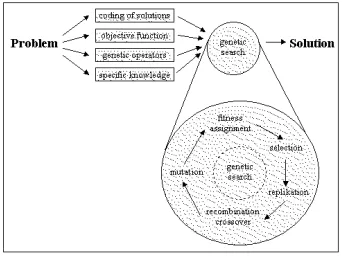
[image:15.595.215.386.206.334.2]

As shown in Figure 2.2, the problem is broken down into the coding of candidate solutions, the objec-tive of the algorithm, genetic operators (mutation, selection), and specific knowledge of the domain — for example — a relationship between variables. A genetic search is performed, consisting of a series of generations, where levels of fitness are assigned to candidates, based on a function related to the objective. A portion of the population at each generation is selected, some are replicated, or recombined through “crossover” of their individual genes. Others have their individual genes mutated. This is repeated for a number of generations.

Figure 2.2: The cycle of generations in a genetic algorithm

2.9.1 The population size

As each generation is produced, the size of the population can grow or shrink depending on constraints placed on the system, usually regarding the required fitness of members of the population. The total number in the population depends on three parameters:

• The number of children

• The number of parents

• The survival of the parents

That is, if the parents survive, the population is determined by population=Σchildren+Σparents, or if the

constraints involve the removal of the parents at each generation, then the final parameter is removed. The rate of survival of the parents, if at all, is generally determined by the “fitness” of an individual candidate when compared to the overall average fitness of the general population, as described in the following section.

2.9.2 The fitness indicator

During each generation, the “fitness” level of each candidate is measured. This is a pre-determined mea-surement to find how closely the candidate matches the ideal or required solution. This fitness assignment is generally performed either through a rank-based fitness assignment (Baker 1985) or as a proportion of the general fitness of the population (Goldberg 1989). As the generations progress, in theory, the fitness of the best candidate available (that is, the difference between itself and the requirements) should tend toward zero, converging on the ideal solution.

Although genetic algorithms are difficult to predict, Holland (1975) made some attempt to quantify the changes in the population after each generation, noting that it was proportional to the fitness of the overall population, and a given set of hypotheses. He also attempted to provide an indicator of the next population, which he eventually quantified as:

E[m(s,t+1)]≥uˆ(s,t)

f(t) m(s,t)(1−pc

d(s)

l−1)(1−pm)

(16)

2.10 GANNs — Genetic Artificial Neural Networks 15

where E[..] is the expected population of a candidate or schema s at the next generation, u(s,t) is the fitness of schema s, f(t)is the average fitness of the population, m(s,t)is the fitness of the current generation, pcis the crossover rate, d(s)is the length of defined bits in the schema or candidate, l is the

length of the schema string, pmis the mutation rate and o(s)is the number of defined bits.

2.9.3 A medical example

Currently, genetic algorithms are already in use as the back-end for a decision support system for cancer therapy, where treatment chromosomes are generated, and evaluated according to a fitness level calculated after running the chromosome through a simulation. Such a system is under trial by a number of clinics in the UK, and is discussed by McCall & Petrovski (1999). Some analysis has gone into the use of ge-netic algorithms to not only determine or test cancer chemotherapy treatments but also to optimise them (Petrovski & McCall 1999).

Genetic algorithms seem well-suited to the problem of warfarin prediction, as their adaptive and flexi-ble qualities lend themselves to proflexi-blems which are not always strictly solvaflexi-ble, and may aid where there are obvious local minima that are not quite optimal, due to their ability to mutate, something which neural networks clearly lack.

2.10 GANNs — Genetic Artificial Neural Networks

Genetic or evolutionary algorithms and neural network algorithms each have their own individual advan-tages. These can, however, be combined to form a GANN — or Genetic Artificial Neural Network, also sometimes known as an Evolutionary Neural Network, or ENN. Here, the evolutionary aspect of the al-gorithm is an additional form of adaption in addition to the learning capabilities inherent in the neural network. These networks can perform a variety of tasks, including weight training, neural network archi-tectural design, self-evaluation and learning of the learning rules, and initial weight selection (Yao 1993).

To apply the genetic aspect to a neural network, each weight can be expressed as a gene of the algorithm. These chromosomes can then be controlled by the genetic algorithm to evolve a number of different neural networks, which can then be evaluated according to a pre-determined (or genetically determined) fitness function. This allows the process of the design to be analogous to a biological process in which the ANN blueprints encoded in chromosomes develop through an evolutionary process(Kus¸c¸u & Thornton 1994).

(17)

Chapter 3

Technical details

“A human being should be able to change a diaper, plan an invasion, butcher a hog, conn a ship, design a building, write a sonnet, balance accounts, build a wall, set a bone, comfort the dying, take orders, give orders, cooperate, act alone, solve equations, analyze a new problem, pitch manure, program a computer,

cook a tasty meal, fight efficiently, die gallantly. Specialization is for insects.” –Robert A. Heinlein

3.1 The concept

Evaluation of the previous methods discussed in Chapter 2 led to the development of number of potential ways to evaluate drug requirements for patients. A number of designs were therefore built incrementally as described in this section. Evaluation of each method is discussed in Chapter 4.

The drug prediction algorithm has a number of specific requirements:

• Accuracy — this is obviously the most important aspect, as the algorithm should be accurate, both in matching an expert’s analysis and predicting the INR level, given a specific situation or patient history.

• Adaptability — the algorithm should be able to change to accommodate variations in drug history, or unusual effects due to changes in medication or other confounding factors.

• Speed — the algorithm should be relatively fast computationally, because it will be running as a back-end to a web-based system, and a long delay is prohibitive in such circumstances (Miller 1968).

In order to satisfy these requirements, we had to first identify the relevant variables in the domain. Secondly, we had to determined a relationship between the variables that would enable the achievement of accurately predicting the dosage and INR readings. The relationship that would be used as the basis of the algorithms would need to be adaptable — allowing for the modification of particular aspects without destroying the overall relationship. The relationship also needed to be simple, so as to allow for a compu-tationally simple and therefore probably fast system. The steps taken to achieve these goals are described in the following sections.

3.2 Identification of variables

The problem of warfarin prediction lends itself to the learning properties of both neural networks and ge-netic algorithms, but first a relationship is necessary to determine warfarin dosage or INR levels.

(18)

3.3 The relationship between variables 17

however, grows exponentially with these factors, and some of them are actually able to be dismissed as irrelevant. This has been observed before, for example, in the study mentioned in Section 2.4 by Vadher et al. (1997), only a few factors were deemed necessary — including the daily dosages, target and actual INR reading, and the rate of change of error — although these could be reformulated in other ways, as discussed below.

In the creation of an adaptive algorithm, one needs to consider changes in the patient’s contributing fac-tors, as these affect how much of an effect the dosage has on the patient. However, these factors can all effectively be taken as the single “filtered effect” of the dose — be it more or less of an effect. This means that, presuming the patient follows a semi-routine lifestyle, the reading would be more or less singularly dependent on the effective dosage received, after being “filtered” through the external factors.

Secondly, the algorithm is meant to be designed for patients that are at least semi-partially stable — for example, they might have INR reading tests twice a week in the most frequent cases. This time period is longer than the effective half-life of warfarin (O’Reilly 1968) and, therefore, should ideally maintain a standard rate — meaning that the length of time between tests is not important, as long as it is longer than the effective half-life of the drug.

The remaining parameters are the dosage taken by the patient on a daily basis, as prescribed by the ex-pert at the time, the reading that this dosage was based on, and the target INR of the patient.

3.3 The relationship between variables

As discussed in Section 3.3, when deciding on a dosage, the expert looks at the INR reading of the patient at the last test, and the target INR of the patient. In addition, they must consider previous readings — to obtain a “feel” for how the patient is doing, and the previous dosages, as a rudimentary guide to the dose that they must now give. From this, we were able to develop the following relationship:

given dosage=α×average dosage

average reading×(target INR−current reading) +β×average dosage (3.1)

This models the relationship that the expert builds in his/her mind in evaluating a patient’s history and current details, and predicting what dose to give. He/she looks at the ratio between the average dosage administered to and the average reading of the patient, as well as the ratio between the INR desired and the one achieved, to obtain a ”difference” to add or subtract from the average dosage given to the patient during their history on warfarin.

α represents the degree of a patient’s response to the deviation from the INR — a low α value signi-fies a cautious adjustment of the dosage, probably due to the patient’s fairly stable history. Similarly, a high

αvalue indicates a stronger response due to the fact that the patient’s readings may be known to be prone to fluctuation, and a change in dosage is immediately necessary. Theβvalue represents how much weight is attributed to the patient’s previous history. Usually this value is around one (to actually give value to the patient’s previous history) — but could be lowered if the patient had received a change in other medication, for example, and therefore their warfarin history would perhaps not be as relevant as that of a stable patient.

3.4 The neural network design

(19)

3.5 The genetic algorithm 18

the Delta rule (Widrow & Hoff 1960), calculating the rate of descent in the neural network incrementally for each example, as in the following equation:

∆wi=η(t−o)xi (3.2)

where∆wiis the change in weight at each example; equal toη(the proportion of weight — that is, the

speed at which it is updated; the learning rate) multiplied by the difference in outputs for each example. The advantage of using the Delta rule is that even if the concept cannot be learned perfectly, it is still able to approximate a potential solution.

The initial weights are randomly set, as they are adjusted very quickly in response to the error encoun-tered when the first example is presented to the algorithm.

3.5 The genetic algorithm

A genetic algorithm was also implemented, because the ability to quickly eliminate poor potential can-didates by predicting the values for the individual patient seemed promising, since the genetic algorithm would hypothetically be able to obtain a result which is almost optimal in a short period of time.

The genes of each of the genetic algorithm’s hypotheses are made up essentially of theαandβvalues in Equation 3.1. Selection is performed on 50% of the population at each generation. The discarded half of the population is created again, using cross-over and splicing of the properties of the selected hypotheses, in an attempt to fine-tune the population. At each generation, the fitness of a given hypothesis is taken to be the average error of the hypothesis’s algorithm, when applied to the patient’s history with the Equation 3.1. There is also a one in ten probability of one of the “inferior” hypotheses mutating; and having its genes randomly altered according to a uniform distribution, in an effort to locate additional ways out of any local minima that the “superior” population may have become trapped in.

3.6 Addition of LMS weightings to form GANNs

As a patient progresses on warfarin, their warfarin requirements change, due to new medication and changes in diet, weight and any number of other factors. A dynamic algorithm needs to take this into account, by deciding whether or not the patient is going through a change, or whether new changes are simply “noise”, due perhaps to the patient missing their medication or a week of illness. The algorithm would then need to adjust weightings for the new readings and dosages accordingly.

A solution is to attempt to focus weights on more recent data, with less importance placed on data the older it becomes. However, simply applying a linear or exponential weighting to the data points will not assist the algorithm in deciding on the noise versus change issue. This is where the concept of a GANN — a Genetic Artificial Neural Network comes in. It has the learning capabilities of a neural network, and the evolving qualities of a genetic algorithm.

In this case, we used LMS — a generalised form of the perceptron, to balance the data historically — and the genetic algorithm to determine candidates that assign various weights to the inputs of the net — that is, the degree of response to the deviation from the INR, and the weight attributed to the average read-ing and dosage of the patient’s history. Values found for these factors help the algorithm make a judgement call as to whether the patient is stable or prone to fluctuation, and how strongly the algorithm should re-spond based on the patient’s history in general, as well as assign these values to the weights given to each of the patient’s data points, respectively.

3.7 Summary

(20)

3.7 Summary 19

(21)

Chapter 4

Experimental results

“Mistakes are a fact of life. It is the response to error that counts.” –Nikki Giovanni

For the experiments, the algorithms are evaluated with respect to their accuracy in dosage prediction, and INR reading prediction. Eleven sets of patient data, each with 16 test points were used for testing. The genetic variants were tested with population sizes of 10, 100, 1,000 and 10,000, and were run with 10, 100, and 1000 generations. The patient data used was obtained with permission, and is included in Appendix A. The data has the dates and names stripped out, leaving the INR readings and the resulting prescribed dosages after each test.

The structure of the genetic algorithms are described in Section 3.5, and more detail is given on the GANN as this chapter progressses. The neural network is also described in Section 3.4.

4.1 Dosage accuracy of each algorithm

After the production of each algorithm, its performance was determined by evaluation of the algorithm with some sample data from patients. The algorithm was trained to learn the history of the patient, to create a dynamic model based on their readings and dosages from their past.

The algorithms, once trained with the patient’s dosage as the desired output — the objective being for the algorithms to learn the practice of the patient’s expert in predicting their dosages, could then be compared to the expert’s predictions to evaluate their performance.

4.1.1 The genetic algorithm — history-based

(22)

4.1 Dosage accuracy of each algorithm 21

0.01 0.1

10 100 1000 10000

Error ratio

Population size

Error rate for varying generations and population sizes of the standard genetic algorithm

[image:22.595.153.447.120.322.2]

"standard 10 generations" "standard 100 generations" "standard 1000 generations"

Figure 4.1: The accuracy of the history-based genetic algorithm

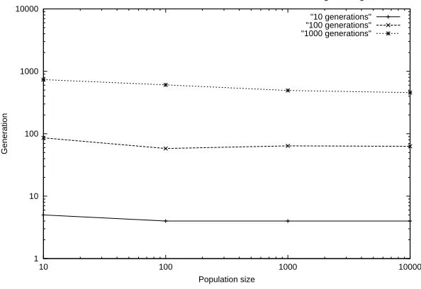
As Figure 4.1 indicates, both the population size and the number of generations aid in reducing the error as they increase in value. However, there is certainly a limit as to how accurately the algorithm can fit its learning patterns to the data. At a population size of 10,000, after 1,000 generations, the error rate is 0.0431 (σ= 0.020), or, in terms of prediction accuracy, the rate is almost 96%. The generation at which the “best” candidate was found was also recorded, and the information is displayed in Figure 4.2.

1 10 100 1000 10000

10 100 1000 10000

Generation

Population size

Generations at which the best candidate was located for the standard genetic algorithm

"10 generations" "100 generations" "1000 generations"

Figure 4.2: Number of generations to find the best candidate

[image:22.595.152.449.448.652.2]

(23)

4.1.2 The neural network

The neural network was also run with the training set, using the patient’s history up to each INR test to predict the expert’s dosage. The results are compared to the standard genetic algorithm, using various generation and population sizes.

0.1

10 100 1000 10000

Error ratio

Population size

Comparison of error rates between the standard genetic algorithm and the neural network

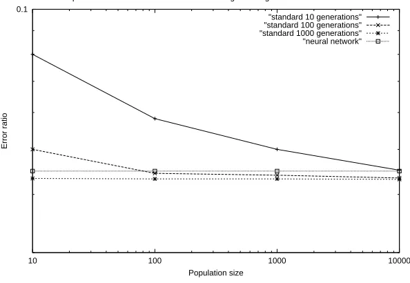
[image:23.595.152.449.188.393.2]

"standard 10 generations" "standard 100 generations" "standard 1000 generations" "neural network"

Figure 4.3: Comparison of genetic algorithm and neural network

The neural network produces an average error rate of 0.0449 (σ= 0.021) over the test cases..

While the genetic algorithm produces less accurate results initially, it very quickly equals the ability of the neural network, without much of an increase in effort and, if the trend continued, would soon pass the neural network in accuracy. In addition, the first tenfold increase in the population size immediately ensures that it beats the neural network from that point on.

4.1.3 The GANN

(24)

0.01 0.1

10 100 1000 10000

Error ratio

Population size

Error rate for varying generations and population sizes of the GANN algorithm

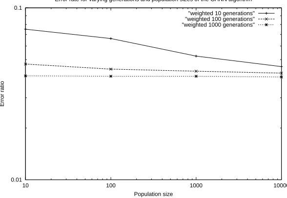
[image:24.595.153.447.119.322.2]

"weighted 10 generations" "weighted 100 generations" "weighted 1000 generations"

Figure 4.4: The accuracy of the weighted genetic algorithm

Figure 4.4 shows that once again, the increase in population size and number of generations helped to lower the error rate of the algorithm when predicting the dosage, although one can see that there is a visible theoretical limit for the data. After 1,000 generations with a population of size 10,000, the error rate is reduced to 0.0396, or approximately 96% in terms of accuracy of prediction.

We also examined the generations required to reach the “best” candidate.

1 10 100 1000 10000

10 100 1000 10000

Generation

Population size

Generations at which the best candidate was located for the GANN algorithm

[image:24.595.152.448.460.664.2]

"10 weighted generations" "100 weighted generations" "1000 weighted generations"

Figure 4.5: Number of generations to obtain the best candidate

(25)

One can then compare the genetic algorithm with its improved weighted version, looking at the differ-ence in error ratios over varying populations. We will show the extreme ends of the range to demonstrate the overall change, when progressing to a population of 10,000 using 1,000 generations.

0.01 0.1

10 100 1000 10000

Error ratio

Population size

A comparison of error rates for the standard genetic algorithm and the GANN algorithm

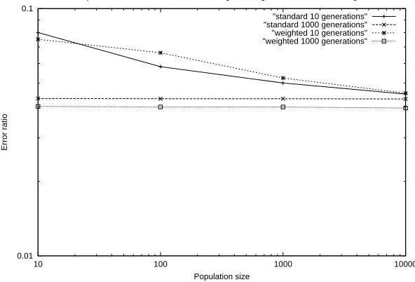
[image:25.595.152.448.170.371.2]

"standard 10 generations" "standard 1000 generations" "weighted 10 generations" "weighted 1000 generations"

Figure 4.6: A comparison of the genetic algorithm with its weighted counterpart

As shown in Figure 4.6, the weighted GANN outperforms the genetic algorithm from the start in each category, and while the standard genetic algorithm provides slightly better performance for some values while using an initial population of size 10, it was likely that this was caused by the confounding pool of candidates to begin with — a local minima was probably located, as the GANN clearly catches up later. However, overall, the GANN certainly performs better than the standard genetic algorithm.

(26)

4.2 Predicting the INR reading 25

0.1

10 100 1000 10000

Error ratio

Population size

Error rates for all three algorithms with varying populations

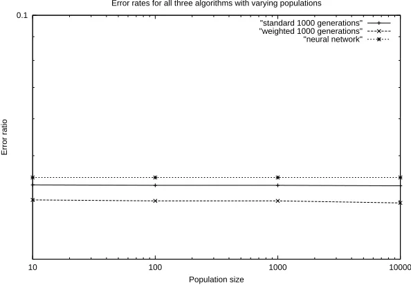
[image:26.595.152.449.116.327.2]

"standard 1000 generations" "weighted 1000 generations" "neural network"

Figure 4.7: A comparison of the best performances of the three algorithms

[image:26.595.205.394.471.522.2]

Clearly, the neural network is conveniently consistent, although is still outperformed by the standard genetic algorithm, which reached its best performance on average at generation 573 (as mentioned earlier in this chapter), with only small improvements before then. The GANN is the superior algorithm, out-performing the standard genetic algorithm by as much as the standard algorithm outperforms the neural network.

Figure 4.8 demonstrates the differences between the algorithms, with their error rates in predicting the INR readings.

Algorithm mean(µ) St. dev. (σ) Neural network 0.0449 0.021 Genetic algorithm 0.0431 0.020 Weighted GANN 0.0396 0.018

Figure 4.8: An analytical comparison of the algorithms’ error rates

As shown in Figure 4.8, it is possible to accurately predict the dosages to between 95.5 and 96 percent accuracy, depending on which machine learning method one chooses to utilise.

4.2 Predicting the INR reading

(27)

The reconfiguration of the algorithms allowed them to learn the following relationship — a rearranged version of equation 3.1.

predicted reading=target INR−average reading

average dosage×

given dosage−(β×average dosage)

α (4.1)

4.2.1 The genetic algorithm — history based

The genetic algorithm was run again with the same parameters, in order to measure its accuracy in INR prediction.

0.1

10 100 1000 10000

Error ratio

Population size

INR prediction error rate for the genetic algorithm

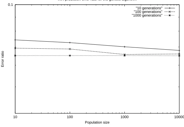
[image:27.595.151.449.257.463.2]

"10 generations" "100 generations" "1000 generations"

Figure 4.9: INR prediction accuracy by the genetic algorithm

As shown, the algorithm shows a general increase in accuracy due to increases in population size, or the number of generations. However, as is visible in the situation where the number of generations was 1000, there is a definite limit to the accuracy of the prediction, as the level of accuracy certainly levels off. Figure 4.10 summarises the prediction of INR readings by the genetic algorithm with 10,000 genera-tions:

Population size Error St. dev.(σ) 10 0.0680 0.027 100 0.0660 0.027 1000 0.0650 0.027

Figure 4.10: A statistical comparison of the genetic algorithm with varying population sizes

4.2.2 The neural network

(28)

0.1

10 100 1000 10000

Error ratio

Population size

INR prediction by the genetic algorithm and the neural network

[image:28.595.153.447.120.322.2]

"10 generations" "100 generations" "1000 generations" "neural network"

Figure 4.11: A comparison of INR prediction accuracy between the genetic algorithm and the neural network

It is also worth noting that the neural network error rate was distributed with a mean of 0.0927, (σ= 0.033).

4.2.3 The GANN

The GANN algorithm was also tested with the same parameters as the first genetic algorithm, with varying population sizes and numbers of generations.

0.1

10 100 1000 10000

Error ratio

Population size

INR prediction error rate for the GANN algorithm

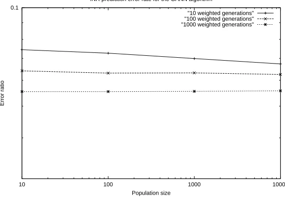
"10 weighted generations" "100 weighted generations" "1000 weighted generations"

Figure 4.12: INR prediction accuracy by the GANN

[image:28.595.153.446.476.679.2]

(29)

Figure 4.13 summarises the prediction of INR readings by the GANN algorithm when run through 10,000 generations.

Population size Error St.dev.(σ) 10 0.0673 0.026 100 0.0625 0.025 1000 0.0557 0.024

Figure 4.13: Statistical comparison of the GANN algorithm with varying population sizes

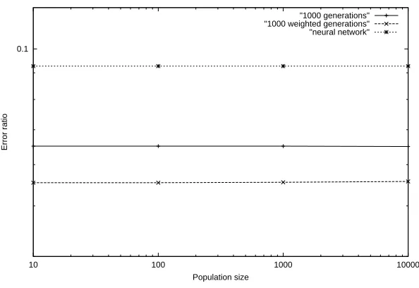
Finally, an analysis of all the algorithms’ performance when predicting the patients’ INR levels is illustrated in Figure 4.14.

0.1

10 100 1000 10000

Error ratio

Population size

Comparison of INR prediction error rate for the three algorithms

[image:29.595.152.449.287.491.2]

"1000 generations" "1000 weighted generations" "neural network"

Figure 4.14: Comparison of all algorithms in predicting INR

[image:29.595.206.397.601.653.2]

As demonstrated in Figure 4.14, the genetic algorithms both outperform the neural network. In addition, the inclusion of the LMS add-on to the genetic algorithm has clearly aided in the prediction of the INR levels, based on changes in the patient’s history.

Figure 4.15 lists the results of a comparison of all three algorithms, with the genetic algorithms using a population of 10,000 and executing through 1,000 generations.

Algorithm mean (µ) St. dev. (σ) Neural network 0.0927 0.033 Genetic algorithm 0.0650 0.027 Weighted GANN 0.0557 0.024

Figure 4.15: An analytical comparison of the algorithms’ error rates in INR prediction

(30)

4.3 Quantitative analysis 29

cannot be compared directly, as different data was used, but is still useful as a guide. Similarly, a study by Byrne et al. (2000) showed that an ensemble of neural networks with 25 parameters was able to present a generalisation error of 0.086, and 0.089 on average for a component network. It would be useful to know which of their 25 parameters were deemed important by their networks, including such factors as patient medication compliance, height, and even marital status.

4.3 Quantitative analysis

The data suggests that there is a difference between the three algorithms, both in predicting the INR read-ings, and prescribing the dosages for each patient. However, statistical analysis is required to determine if this difference is statistically significant. A one-tailed test is required to determine whether one algorithm is statistically superior to another, where the level of significance is set toα=0.05.

4.3.1 Predicting the dosage

A one-way analysis-of-variance was applied to the results of the three algorithms in predicting the dosage, which demonstrated that the means for the algorithms were not significantly different (F2,30= 0.215, p =

0.807). This shows that while there is no significant difference, there is likely a link between their taget outputs, and is probably due to the fact that all three algorithms were trying to aim for similar results, at-tempting to emulate or “mimic” the dosages prescribed by the patient’s current expert. We would, however, expect to find differences if the same experiment was performed with live patient tests, as the algorithms would change to aim for the ideal dosages, rather than those prescribed by the patient’s doctor.

4.3.2 Predicting the INR

A one-way analysis-of-variance was applied to the three algorithms, to establish that the means for the algorithms were significantly different (F2,30= 5.073, p<0.0013). Since there is a difference, a post-hoc

Bonferroni Correction is required for comparison. The required value for p (<0.05) is divided by the number of comparisons (three) to maintainα, so only those T-Tests with p<0.0167 will be significant.

A paired T-Test was then performed on each pair of algorithms, in order to establish where the signifi-cant difference(s) lay. Firstly, the genetic algorithm was compared to the neural network. As demonstrated in the results, the genetic algorithm (µ = 0.0650,σ= 0.027) outperformed the neural network (µ = 0.0927,

σ= 0.033). This difference is considered to be statistically significant, with T9=1.2254, p<0.0111. The

two genetic algorithm variants were also compared. The standard genetic algorithm (µ = 0.0650,σ= 0.027) was outperformed by the GANN (µ = 0.0557,σ= 0.024). This difference can also be considered statis-tically significant, with T9=7.6492, p<0.006. Finally, the neural network is compared to the GANN,

where the GANN is significantly different (and clearly superior) than the neural network, with T9=1.1666,

p<0.0002.

4.4 Summary of results

First and foremost, our results demonstrated that it is both relatively simple and realistic to use computer-based methods to predict the effects of warfarin, and thereby to prescribe warfarin dosages. Each method evaluated was able to both accurately match the expert’s predictions, and accurately predict the patient’s resultant INR, when provided with a particular dosage. This was performed solely by using the dosage and INR reading history of the patients, and utilising the method described in Chapter 3.

(31)

4.4 Summary of results 30

(32)

Chapter 5

Discussion

5.1 Positive aspects

As shown in Chapter 4, the results are very promising. Each of the algorithms was able to predict both dosage and INR with a high level of accuracy. It is clear from the results, that the algorithms are quickly able to reach an acceptable level of accuracy, even with small populations and few numbers of generations.

As noted in Chapter 3, each data set was composed of only 16 points. It is common for this to repre-sent only six weeks to six months of data. We hope that the results thus far are indicative of an even higher accuracy rate when more data points per patient are entered, as many have years of data available on which to train the algorithms.

It was also interesting to note that, when the algorithms were trained using the expert’s given dosage as the output, they were able to follow and match the dosaging patterns of the experts with high accuracy. Not only does this mean that the algorithms can be trained to be nearly equal with experts in the field, but that the experts were reasonably consistent in their dosaging. If they were inconsistent, the algorithms would have failed to find a pattern that matched all cases with marginal error. We would hope that this is generally the case, as subconscious fears of over- or under-coagulating could cause doctors to under- or over-prescribe, potentially causing difficulties for patients, or at the least, putting them at greater risk.

5.2 Shortcomings

A shortfall of the genetic variants is the time required to achieve the high accuracy. On the machine used to test the results (AMD Athlon(tm) XP 1600+, 512mb RAM), the standard genetic algorithm took almost an hour and a half to execute, while the GANN took over three hours. However, using the lower population sizes and numbers of generations decreased the time by an order of magnitude for each similarly propor-tioned reduction of as seen in the results in Chapter 4. Therefore, even in a few seconds, the algorithms are able to reach reasonably high levels of accuracy. However, in the future as computers increase in speed, we might simply be able to increase the number of generations and the population size to increase the accuracy as demonstrated, although this accuracy rate would inevitably reach a limit.

5.3 Lack of data

(33)

5.3 Lack of data 32

examples of bleeding or irregularities; however, more data would certainly have been useful. Unfortunately, delays in the process of obtaining the ethical approval for alternate data collection were too long.

(34)

Chapter 6

Further work

6.1 Improvements

While the algorithms have demonstrated their ability to both accurately predict INR readings, and prescribe warfarin dosages, there are still areas where they may be improved upon.

In the future, an investigation of the genetic algorithms could be undertaken in order to evaluate differ-ent rates of mutation. The currdiffer-ent rate of mutation (one in ten) was chosen after an initial experimdiffer-ent to try and obtain a rough value for for the mutation rate. However, recent evaluations have shown that, in some circumstances, the use of a mutation rate of 1/l can produce favourable rates of success, where l is the

length of bits of each bit string (B¨ack 1993). However, we predict that this would only produce very minor improvements at best, and is really a case for optimisation of algorithms, rather than selection of which algorithm to use.

The speed of the algorithms is another area where our work could be progressed. As described earlier, the genetic algorithms required a significant amount of time time run, but delivered only a slight improve-ment. This improvement is, however, clearly achievable and therefore, ideally, we would like to reach the greatest level of accuracy attainable. While this problem may be solved with faster computers, it would be useful to investigate additional standardised initial base values for the genetic algorithms, obtaining a form of average relationship between the general population of patients’ INR readings and their dosages. This relationship would also be helpful for prescribing warfarin to patients when they initially begin taking warfarin, as there would be an accurate guide to consult.

6.2 Fuzzy Logic

(35)

6.3 Additional data 34

6.3 Additional data

Ethical approval for further data should soon be available through the Cardiology Department of Christchurch Public Hospital. It would be useful to re-evaluate the algorithms with more data to ensure the algorithms’ validity, and to see how they might perform in further unusual situations, such noisy data, bleeding, patients just beginning to take warfarin, and other irregularities.

6.4 In hospital trials

The next phase of our work would most likely involve obtaining ethical approval for live patient trials; testing the algorithm in a real situation with patients currently on warfarin. Such a trial would have to be supervised by a patient’s current doctor or physician. The benefits would include the ability to observe the algorithm in a real world environment, to see how it copes or performs with actual patients and their data, and how accurately it adapts as their warfarin needs change. The data collected from these trials would be invaluable for further testing of the algorithm, and would also serve as a form of validating the method of prediction used.

6.5 A web-based implementation

The project proposed by David Shaw focused on a web-based solution for patients, who could log on to a web-site and have the site prescribe warfarin based on their dosage and reading history. Such a site could help ease the problems caused by the often inaccurate prescription of warfarin. It would also allow the patients to help themselves in monitoring their levels and become a part of their own medical team.

The algorithm itself can easily be placed in the back-end of the website, attached server-side to an in-dividual page. The data could be retrieved from a database of the patient’s history, uniquely identified by the patient’s ID — retrieved only after authentication of the patient via a separate database. This would maintain the privacy required, as well as avoiding the potential for malicious users to corrupt sensitive patient data.

Running the algorithm server-side almost certainly implies a potential delay in the processing of the data and the availability of the results to the user. However, a simple on-screen indicator of the delay is deemed sufficient according to the guidelines outlined in a paper by Miller (1968). The patient will wait only a matter of seconds, as opposed to the hours required to process data through an expert via laboratories.

6.6 Development of an algorithm for other medications

(36)

Chapter 7

Conclusion

We investigated the issues involved in the prediction of the effects of warfarin, and how to accurately prescribe warfarin dosages to ensure patients meet their target range.

We found that warfarin affects every patient in a slightly different way, and that a dynamic, adaptive model is needed to accurately model a patient and their dosaging history. We also determined that many external factors could be grouped to ultimately imply an altered “effective” effect of the warfarin on the individual patient.

Three machine learning techniques were evaluated as to their ability to accurately model the patient’s history, and to accurately predict and prescribe warfarin based on what they had learned. The evaluation focused on their ability to mimic an expert in predicting dosages, and then from given dosages, predicting patient INR values as a result of these dosages.

A simple neural network perceptron model evaluated well, predicting dosages with an average 95.5% accuracy. A genetic algorithm was able to predict up to 95.7%, and a weighted genetic artificial neural network performed the best, with an average 96% accuracy. When predicting INR readings, the neural network reached 91.1%, the genetic algorithm was able to obtain 93.5%, and the GANN scored 94.4%.

Overall, there was not much difference between the algorithms, with all predicting rather highly, al-though the genetic variants always surpassed the neural network on each test-case. The weighted GANN was also able to out-perform the genetic algorithm. However, they are significantly higher than current levels of accuracy achieved by experts.

The result of this report demonstrates that it is possible to accurately predict the effects of warfarin, and accurately prescribe dosages based on the history of a patient. It is also possible to adapt for the individual differences between patients, and to adapt to changes that any patient may go through that affect their warfarin requirements.

Acknowledgments

(37)

Appendix A

Below is some sample patient data, with their INR readings and consequent warfarin dosages.

readings = {2.3,2.0,1.9,2.9,2.1,2.9,2.5,2.1,3.7,2.6, 2.7, 2.6, 2.8, 2.5, 2.6, 2.7} dosages = {2.5,2.5,3.0,2.5,3.0,2.5,2.5,3.0,2.5,3.0,2.75,2.75,2.75,2.75,2.75,2.75}

readings = { 2.3, 2.7,3.2, 2.5, 2.6, 2.1, 2.8,1.9, 2.8,1.9,2.2, 3.2,2.4,2.9,2.8,2.3} dosages = {2.75,2.75,2.5,2.75,2.75,2.75,2.75,3.0,2.75,3.0,3.0,2.75,3.0,3.0,3.0,3.0}

readings = {1.6,1.5,1.7,2.0,2.1,2.5,2.6, 3.3, 3.0,2.0,1.8,2.4,2.7,2.8,3.7,3.5} dosages = {3.0,3.0,3.0,3.0,3.0,3.0,3.0,2.75,2.75,3.0,3.5,3.0,2.5,2.5,2.0,2.0}

readings = {2.8,2.2,2.1,2.0,2.3,2.3,2.4,2.3,2.3,2.5,2.8,2.5,1.7,2.1,2.2,2.3} dosages = {2.5,2.5,2.75,3.0,3.0,3.0,3.0,3.0,3.0,3.0,3.0,3.0,3.5,3.5,3.5,3.5}

(38)

Bibliography

B¨ack, T. (1993), ‘Optimal Mutation Rates in Genetic Search’, Proceedings of the Fifth International

Con-ference on Genetic Algorithms pp. 2–8.

Baker, J. (1985), ‘Adaptive Selection Methods for Genetic Algorithms’, Proceedings of an International

Conference on Genetic Algorithms and their Application, Hillsdale, New Jersey pp. 101–111.

Beckett, L., Rosner, B., Roche, A. & Guo, S. (1992), ‘Serial changes in blood pressure from adolescence into adulthood’, American Journal of Epidemiology 135, 1166–1177.

Breckenridge, A. (1977), ‘Interindividual differences in the response to oral anticoagulants’, Drugs

14, 367–375.

Byrne, S., Cunningham, P., Barry, A., Graham, I., Delaney, T. & Corrigan, O. I. (2000), ‘Using Neural Nets for Decision Support in Prescription and Outcome Prediction in Anticoagulation Drug Therapy’,

In-telligent Data Analysis In Medicine and Pharmacology, a Workshop at the 14th European Conference on Artificial Intelligence .

Camargo, F. A. (1990), Learning Algorithms in Neural Networks, Technical Report CUCS-062-90, New York, NY, 10027.

Cook, N., Gillman, M., Rosner, B., Taylor, J. & Hennekens, C. (2000), ‘Combining annual blood pres-sure meapres-surements in childhood to improve prediction of young adult blood prespres-sure’, Statistics in

Medicine 19, 2625–2640.

Copplestone, A. & Roath, S. (1984), ‘Assessment of therapeutic control of anticoagulation’, Acta

Haema-tolology 71, 376–380.

Cosmi, B., Palareti, G., Moia, M., Carpenedo, M., Pengo, V., Biasiolo, A., Rampazzo, P., Morstabilini, G. & Testa, S. (2000), ‘Assessment of patient capability to self-adjust oral anticoagulant dose: a multi-center study on home use of a portable prothrombin time monitor (COAGUCHECK)’, Haematologica

85, 826–831.

Doble, N. & Baron, J. (1987), ‘Anticoagulation control with warfarin by junior hospital doctors’, Journal

of the Royal Society of Medicine 80, 627.

Duxbury, B. (1982), ‘Therapeutic control of anticoagulant treatment’, British Medical Journal 284, 702– 704.

Goldberg, D. (1989), ‘Genetic algorithms in Search, Optimization, and Machine Learning’, Reading,

Mass.: Addison-Wesley .

Gurney, K. (1996), An Introduction to Neural Networks, UCL Press.

Hoffer, E. (1975), ‘A computer-based information system for managing patients on long-term oral antico-agulants’, Computational Biomedical Research 8, 573–579.

An Adaptive Computer Based System for the Prescription of Warfarin