Two temperate sub Neptunes transiting the star EPIC 212737443

Advance Access publication 2019 June 14

Two temperate sub-Neptunes transiting the star EPIC 212737443

Mahesh Herath,

Tobias C. Hinse ,

John H. Livingston ,

Jes´us Hern´andez,

Daniel F. Evans,

Robert Wells ,

Saraj Gunesekera,

Jeremy Tregloan-Reed,

Markus Rabus ,

Jesper Skottfelt,

Martin Dominik ,

Uffe G. Jørgensen,

Chandana Jayaratne

and Cuc T. K. L´y

1_{Department of Astronomy, Arthur C. Clarke Institute for Modern Technologies, 0272 Moratuwa, Sri Lanka} 2_{Department of Physics, Astronomy and Space Science Unit, University of Colombo 00300, Sri Lanka}

3_{Department of Astronomy and Space Science, Chungnam National University, Daejeon 34134, Republic of Korea} 4_{Department of Astronomy, University of Tokyo, 7-3-1 Hongo, Bunkyo-ku, Tokyo 113-0033, Japan}

5_{Instituto de Astronomia, Universidad Nacional Autonoma de Mexico, Ensenada, B.C., Mexico} 6_{Astrophysics Group, Keele University, Staffordshire ST5 5BG, UK}

7_{School of Mathematics and Physics, Queens University Belfast, University Rd, Belfast BT7 1NN, UK}

8_{Centro de Astronom´ıa (CITEVA), Universidad de Antofagasta, Avenida U. de Antofagasta 02800, Antofagasta, Chile} 9_{Las Cumbres Observatory Global Telescope, 6740 Cortona Dr., Suite 102, Goleta, CA 93111, USA}

10_{Department of Physics, University of California, Santa Barbara, CA 93106-9530, USA}

11_{Department of Physical Sciences, Centre for Electronic Imaging, The Open University, Milton Keynes MK7 6AA, UK}

12_{Niels Bohr Institute & Centre for Star and Planet Formation, University of Copenhagen, Øster Voldgade 5, DK-1350 Copenhagen, Denmark} 13_{Centre for Exoplanet Science, SUPA School of Physics & Astronomy, University of St Andrews, North Haugh, St Andrews KY16 9SS, UK} 14_{Department of Physics, Quy Nhon University, 590-000 Quy Nhon, Socialist Republic of Vietnam}

Accepted 2019 June 6. Received 2019 June 5; in original form 2019 January 10

A B S T R A C T

We report the validation of a new planetary system around the K3 star EPIC 212737443 using a combination ofK2 photometry, follow-up high-resolution imaging and spectroscopy. The system consists of two sub-Neptune sized transiting planets with radii of 2.6R_⊕and 2.7R_⊕, with orbital periods of 13.6 and 65.5 d, equilibrium temperatures of 536 and 316 K, respectively. In the context of validatedK2 systems, the outer planet has the longest precisely measured orbital period, as well as the lowest equilibrium temperature for a planet orbiting a star of spectral type earlier than M. The two planets in this system have a mutual Hill radius ofRH =36, larger than most other known transiting multiplanet systems, suggesting the existence of another (possibly non-transiting) planet, or that the system is not maximally packed.

Key words: techniques: photometric – techniques: spectroscopic – eclipses – planets and satellites: detection.

1 I N T R O D U C T I O N

TheKepler mission (Borucki, Koch & Basri 2010) enabled the discovery of exoplanets at a rate unlike any mission before. The data collected byKeplerhave uncovered a large variety of planetary systems, with more continuing to be found (e.g. Mayo et al.2018b). TheK2 mission utilized the same spacecraft to observe different fields along the ecliptic plane for 80 d each. This time baseline limited theK2 mission to detecting planets with orbital periods shorter than 45 d on average. Among the small number of confirmed planets with long orbital periods measured by theK2 mission, the longest until now was K2-118b (Dressing et al.2017); this planet has a period of 50.9 d and a size of 2.49R⊕. Another long-period planet

_{E-mail:[email protected](MH);[email protected](TCH)}

is K2-263b (2.41R⊕) with a 50.8 d orbit (Mortier et al.2018); K2-263b remains the only planet from the mission with a period greater than 45 d that has a precisely measured mass ((14.8±3.1)M_⊕). The HIP41378 system (Vanderburg et al.2016b) is thought to contain three planets (planetsd,e,andf) with likely periods of 156, 131, and 324 d, respectively. Multiple transits were observed for these three planets throughK2 campaigns 5 and 18, though their periods are yet to be precisely determined (Becker et al. 2018; Berardo et al.2018). The EPIC 248847494 system fromK2 campaign 14 was found to have a single transit event lasting 54 h, which was revealed to be a possible Jupiter-like planet (1.11RJup) through

photometric analysis and radial velocity observations (Giles et al. 2018). This object has an estimated orbital period of 3650 d, and is classified as a planet candidate due to having just one observed transit. If confirmed, it would be the longest period transiting exoplanet.

2019 The Author(s)

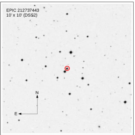
Figure 1. Display of a 10×10 arcmin finder chart of EPIC 212737443 (the red circle) obtained from the digital sky survey (DSS2). The star towards south-east is catalogued as EPIC 212737293 and has an angular separation of 17 arcsec. The proper motion of EPIC 212737293 (GaiaDR2) is μα= −2.017 mas yr−1, μδ=0.037 mas yr−1 at a distance of around

2400 pc. Therefore, the two stars are unrelated.See electronic version for colours.

In this work, we report the validation of two sub-Neptune sized planets orbiting a K3-type star at a distance of 347 pc. The outer planet of this system has the longest precisely measured orbital period amongK2 planets (P=65.5 d), and this is the only confirmed

K2 multiplanet system with a long-period planet showing two or more transits. In Section 2, details of the K2 data reduction and ground-based observations are given. Sections 3.1 and 3.2 outline details of the transit identification and fitting procedure used to characterize each planet candidate. In Section 3.3, we review host-star properties as obtained from a previous study. The stellar parameters are derived in Sections 3.4–3.7. A planet validation analysis by means of a false positive probability (FPP) is presented in Section 4, as well as a dynamical analysis in Section 5. The paper is concluded with a discussion of our findings and a summary in Sections 6 and 7, respectively.

2 O B S E RVAT I O N S

2.1 K2 photometry

Due to the failure of two reaction wheels, theKeplerspacecraft was re-purposed as theK2 mission in 2014 (Howell et al.2014). Recently, in 2018 October theKepler telescope was decommis-sioned. EPIC 212737443 was observed duringK2 campaign 6 for approximately 80 d between 2015 July 13 and 2015 September 30. Fig.1shows a portion of sky centred on the star. The motion of stars over pixels of variable sensitivities caused by the rotation of the spacecraft around its boresight angle can show apparent variations in stellar brightness. A method to remove these systematic variations was devised by Vanderburg & Johnson (2014), which we will describe in brief. An aperture is placed around the target star, which is defined as either an approximately circular pixel region,

Figure 2. TheK2 image (9×8 pixels) summed from all postage stamp frames of EPIC 212737443 (Vanderburg & Johnson 2014). The image shown is rotated 7.5 deg east of north (top of the image). Here, the optimal photometric aperture is overplotted in red around the target, with the green dot indicating the centre of the flux distribution. The nearest field star is located a fewK2 pixels away towards the south-east direction.See electronic version for colours.

or a region of pixels determined by the pixel response function. The best aperture is found by optimizing the photometric precision of the corrected light curve. The red region in Fig. 2shows the best aperture chosen in this work and avoids any light contribution from the nearby field star. The flux inside the optimal aperture is decorrelated from position-dependent trends to produce light curves that are available in the Mikulski Archive for Space Telescopes (MAST1_{). The target light curve was retrieved from MAST and we}

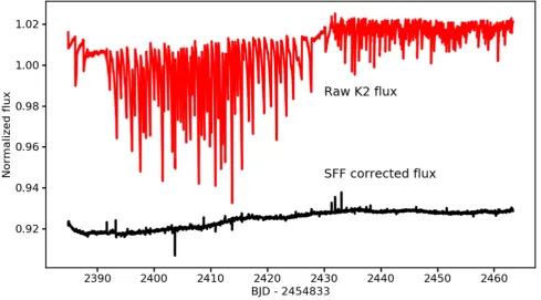
removed long-term time-dependent trends by fitting and subtracting a cubic spline with knots spaced 0.75 d apart. Fig.3shows the raw and detrendedK2 light curve for EPIC 212737443.

2.2 Speckle imaging

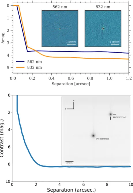
Additional data were obtained from the NASA Exoplanet Star and Speckle Imager (NESSI) at the Kitt Peak National Observatory. We collected data following the procedures described in Howell et al. (2011). Speckle-interferometric observations were conducted simultaneously in the ‘blue’ and ‘red’ bands centred at 562 (width= 44 nm) and 832 nm (width =40 nm), respectively (Scott, Howell & Horch2016), at a frame rate of 25 Hz. After data reduction following Howell et al. (2011), we obtained diffraction-limited target images with dimensions of 4.6 × 4.6 arcsec (Horch et al. 2009, 2012, 2017). Using concentric annuli centred on the target, we found the background sensitivity limits were estimated as described in Howell et al. (2011). Finally, a contrast curve was produced by fitting a cubic spline to the smoothed 5σ sensitivity limit. The top panel of Fig.4shows the contrast curve derived from NESSI observations.

2.3 Lucky imaging

We obtained high-resolution images with a lucky-imaging camera on the night of 2018 May 3 in order to search for nearby stars

1_{https://archive.stsci.edu/}

Figure 3. The rawK2 light curve for EPIC 212737443 (red) with the position-dependent trends removed (black) using the methods in Vanderburg & Johnson (2014).See electronic version for colours.

potentially contributing with contaminating light, as well as detect potential bound companions. The observations were conducted as part of the 2018 MiNDSTEp2_{campaign using the two-colour}

instrument (TCI) at the Danish 1.54-m Telescope at ESO/La Silla Observatory. Each TCI consists of a 512 ×512 pixel Electron Multiplying CCD (Andor, iXon + 897) capable of imaging si-multaneously in two colours with a field of view (FOV) of about 45×45 arcsec2_{. A detailed description of the instrument and lucky}

imaging reduction pipeline can be found in Skottfelt et al. (2015). The observations and data reduction were carried out using the method outlined in Evans et al. (2016, 2018), which is briefly described here. The target was observed for 900 s at a frame rate of 10 Hz. The raw data were reduced automatically by the instrument pipeline that performs bias and flat frame corrections, removal of cosmic rays, determination of the quality of each frame, and frame re-centring with the end product being 10 sets of stacked frames ordered by quality. This is then run through a custom star detection algorithm (Evans et al.2016,2018) that is designed to detect close companion stars that may not be fully resolved. At this point, we would like to stress that due to an observer error the TCI field was centred on the brighter background star EPIC 212737293. This does not, however, affect the images. No close companion stars were detected in the lucky imaging data. The only star visible within the TCI FOV is the well-resolved EPIC 212737293 towards the south-east direction at a distance of around 17 arcsec, and it falls outside the K2SFF pixel aperture. The contrast curve for the LI data can be seen in Fig.4.

2_{http://www.mindstep-science.org/}

2.4 Archival TripleSpec spectroscopy

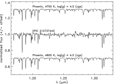
We used a near-infrared (NIR) spectrum of EPIC 212737443 obtained by Dressing et al. (2017; see their fig. 23) using the TripleSpec instrument (Herter et al. 2008) installed at the 20-inch Palomar–Hale Telescope. The spectrum was obtained from the ExoFOP-K23 _{page for the target star. The spectrograph was}

operated in the fixed (east–west) 1×30 arcsec slit-mode yielding a simultaneous coverage of wavelengths between 1.0 and 2.4μm (covering theYJHKbands) at a spectral resolution of 2500–2700 sampled at 2.7 pixels per resolution element. Core details on the reduction of the spectrum and the corrections that were applied such as the removal of telluric absorption features can be found in Dressing et al. (2017).

2.5 Broad-band archive photometry

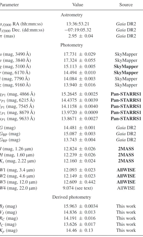
We use archive photometric archive data spanning the wavelength region from ultraviolet to infrared. Apparent magnitudes from multiband photometry are obtained from 2MASS (Skrutskie et al. 2006) [J,H,Ks], Pan-STARRS DR1 (Chambers et al.2016) [g,r,

i,z,y], Sky-Mapper4_{(Wolf et al.2018) [u,v,g,r,i,z], AllWISE}

(Wright et al. 2010) [W1, W2, W3, W4], and Gaia DR2 (Gaia Collaboration2018b) [G,GBP,GRP]. All data except for the

Sky-Mapper data were retrieved and compiled via the ViZieR service. We note that the AllWISEW3 andW4 magnitudes have significantly less photometric precision compared to the other two measurements.

3_{https://exofop.ipac.caltech.edu/k2/edit target.php?id = 212737443} 4_{http://skymapper.anu.edu.au/}

Figure 4. Top panel: Contrast sensitivity curve (mag) versus separation of EPIC 212737443 from the two reconstructed WIYN/NESSI images (inset).Bottom panel: Contrast curve for EPIC 212737443 as obtained from the Danish 1.54-m telescope and spanning a radius of 10 arcsec from the centre (cross-hair). The inset figure (inverse logarithmic scale) shows the 45×45 arcsec TCI field of view (red camera) including the nearest star EPIC 212737293 located at a distance of about 17 arcsec.See electronic version for colours.

In particular, theW4 magnitude is only an upper limit with a signal to noise of less than 2. No photometric data from the Sloan Digital Sky Survey exist for EPIC 212737443.

3 DATA A N A LY S I S

3.1 Transit detections

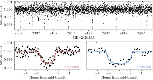
A transiting planet candidate with a 13.6 d period was identified in theK2 light curve by Pope, Parviainen & Aigrain (2016) and again by Barros, Demangeon & Deleuil (2016) for this system. We used the box least square (BLS) algorithm (Kovacs, Zucker & Mazeh2002) with a signal detection efficiency (SDE; Ofir2014) to confirm the existence of this candidate. The BLS search yielded a 13.6 d signal with a transit depth of 1000 ppm (parts per million) and SDE of 11. We masked the transits identified from the first BLS iteration and ran the BLS algorithm again over the residual data. The second BLS iteration revealed a signal with a period of 65.5 d with SDE=7. Upon visual inspection of the light curve, we identify two transit events at 2394.78 (BJD-2454833) and 2460.44, with each transit having a depth of 1100 ppm.

3.2 Transit modelling

We used thePYTHON packageBATMAN5(Kreidberg2015) to model the transits (Mandel & Agol2002). For computational efficiency, we fitted the models to regions of three transit durations (3 ×

T14) centred on each transit. The free parameters used to compute

the models include the planet–star radius ratio Rp/R, the scaled

semimajor axis a/R, the impact parameter b= acosi/R where

iis the orbital inclination to the line of sight, the epoch of first transitT0, the orbital periodP, and two limb-darkening coefficients

(q1,q2) from Kipping (2013) assuming a quadratic limb-darkening

law. Monte Carlo sampling of the stellar parameters was used to obtain the distributions of the limb darkening-coefficients from an interpolated grid based on the tabulated parameters of Claret, Hauschildt & Witte (2012), which were then used for Gaussian priors on the limb-darkening coefficients. The limb-darkening co-efficients were determined based on stellar atmospheric properties as derived in this work (see Section 3.5). Uniform priors were used for all other parameters. In addition, we fitted for the logarithm of the Gaussian errors (logσ) and a constant out-of-transit baseline offset. For parameter estimation, we used an affine-invariant Monte Carlo Markov Chain (MCMC) implemented within theEMCEE PYTHON package (Foreman-Mackey et al. 2013) to sample the posterior distributions of the aforementioned transit model parameters. The MCMC was run for 5000 steps using 100 walkers and a burn-in phase of 2000 steps. We computed the autocorrelation time of each parameter to ensure that we collected at least several thousand effectively independent samples after burn-in. The evolution of the MCMC chain populations was qualitatively monitored by generating trace plots for each parameter. The chains showed convergence after about 600 steps.

The fitted parameters were used to derive the inclinationi, and transit duration T14. Initially, we did not impose a prior on the

stellar density (ρ) and derived its value through the transit fits themselves. The mean stellar densities from the fits for planets

bandcwere 3.46+₋12..3735and 3.96+ 1.76

−2.67 g cm−3, respectively. These

values are in excellent agreement with each other (0.14σ), and with the independently derived value for mean stellar density of ρ=3.190+₋00..256250 g cm−

3_{. We repeated our parameter estimation}

calculations with a Gaussian prior based on the stellar density derived in Section 3.8. In addition, we did not detect any transit timing variations in this system. Fig.5gives the folded light curves with their respective best-fitting models for planetsband c. We report the median and 68 per cent credible interval of the resulting posteriors.

For planetc, we fitted each transit separately, using a uniform prior for the orbital period and assuming both circular and eccentric orbits. We then compared the resulting posteriors from each fit. The duration and depth agreed to within 0.06σ and 0.27σ for all posteriors (both eccentric and circular orbits). We repeated the experiment using a Gaussian prior on the mean stellar density, the value of which is based on our results in Table 3. In this case, the posterior distribution of the orbital period peaked near 65 d. Under the assumption that the transits are from two different objects, we then computed the minimum orbital periods necessary to replicate the observations in our data. Using the mid-transit time of each eclipse with the start and end points of the photometry, we determined that the shortest period that would show a single transit is 68.6 d. We then used the radius derived for each transit to

5_{https://www.cfa.harvard.edu/ lkreidberg/batman/}

Figure 5. Top panel: The reduced light curve for EPIC 212737443 with the transits marked using the red and blue ticks.Bottom panels: The phase-folded transit for each planet overlaid with the best-fitting transit model in red and blue for planets b and c, respectively.See electronic version for colours.

estimate planet masses via the empirical mass–radius relationship of Weiss & Marcy (2014). Following Weiss et al. (2018), we found the ratio of periods (P2/P1) corresponding to a Mutual Hill radius

of 3.5, which is the theoretically determined stability criterion for the minimum space between two planets (Wisdom 1980). This presented a scenario in which two equally sized planets with periods of 68.6 and 80.2 d can recreate the two transits seen in our data set. Assuming that these orbits are circular (e=0) with equatorial transits (b=0), we computed the transit durations using the periods and their semimajor axes. The durations were larger (0.2320 ± 0.06 and 0.2450± 0.07 d) by a factor of 0.68σ and 0.72σ than the durations of the observed transits (0.190±0.016 and 0.192±0.022 d). The durations differ by a factor of 0.15σ between transits as opposed to the 0.06σdifference in our observed transits. However, the durations become indistinguishable between orbits for values of e>0 andb>0.

3.3 Preliminary stellar classification

An initial characterization of EPIC 212737443 was presented by Huber et al. (2017) based on the classification of 138–600 stars in

K2 campaigns 1–8. The result constitutes the Ecliptic Plane Input Catalog (EPIC6_{). The single-star characterization is based on a}

simulated synthetic stellar population obtained from theGalaxia

model (Sharma et al. 2011). The model is obtained by means of calibration of the observed J-band distribution of a sample of targets in theKepler field with well-determined stellar prop-erties obtained from asteroseismology and spectroscopy (Huber et al. 2014). Stellar properties are then inferred from posterior probabilities using the synthetic stellar population as a prior in conjunction with archive broad-band photometry and kinematics for

6_{http://vizier.u-strasbg.fr/viz-bin/VizieR?-source = J/ApJS/224/2}

Table 1. Stellar properties of EPIC 212737443 from the Huber et al. (2017) EPIC stellar classification from K2 campaigns 1–8. Parameter values were obtained from the EPIC catalog retrieved via the VizieR (http://vizier.u-strasbg.fr/viz-bin/VizieR) service. We note that the ExoFOP https://exofop.ipac.caltech.edu/k2 data base has incomplete information. The KepFlag=JHK indicates the Kepler magnitudeKpwas calculated from 2MASSJHKsphotometry, which we have repeated in this work in order to derive an uncertainty estimate based on Monte Carlo error propagation.

Parameter Value Source

Teff(K) 4542+₋149298 Huber et al. (2016)

logg(cgs) 4.708+₋₀0_..088₀₄₀ Huber et al. (2016) Radius,R(R) 0.57₋+₀0._.054₀₉₅ Huber et al. (2016) Mass,M(M) 0.615₋+₀0._.049₀₈₉ Huber et al. (2016) [Fe/H] (dex) −0.473+₋₀0_..300₂₅₀ Huber et al. (2016) Distance (pc) 290.8+₋27₆₈._.3₇ Huber et al. (2016) Density,ρ(cgs) 3.22₀+_.5121.49 Huber et al. (2016)

E(B−V) (mag) 0.037+₋₀0_..035₀₁₃ Huber et al. (2016)

Kp(mag) 14.46±0.13 this work

μα(mas yr−1) −54.1±2.5 Huber et al. (2016)

μδ(mas yr−1) 25.8±3.0 Huber et al. (2016)

Catalogue s-flag rpm Huber et al. (2016) Catalogue

KepFlag

JHK Huber et al. (2016)

Catalogue K-flag 1 Huber et al. (2016)

each catalogue star. Stellar masses are predicted from interpolation of tabulated isochrones obtained from thePadovastellar evolution data base. Stellar properties of EPIC 212737443 as obtained by Huber et al. (2017) are listed in Table1. The characterization of EPIC 212737443 uses the reduced proper motion (Gould & Morgan 2003) and 2MASSJHKsphotometry (Skrutskie et al.2006). We find

theJ−Kscolour to be 0.664±0.035. TheJ-band reduced proper

Figure 6. Observed and normalizedJ-band TripleSpec spectrum of EPIC 212737443 (middle) compared to Phoenix synthetic spectra fixed at logg= 4.5 (cgs).

motion (RPMJ) is calculated to be 6.373±0.026 mag using recent

GaiaDR2 astrometry data (Section 3.4). Qualitatively, the (J−Ks,

RPMJ) measurements classifies EPIC 212737443 as a dwarf-star

(see their fig. 6; Huber et al.2017). For this particular population, loggseems to be well constrained to within a relatively narrow interval of logg∈[3.5, 5] withTeffspanning from 3500 to 8000 K.

These parameter ranges are consistent with what is expected for dwarf stars from theoretical considerations.

We note that Huber et al. (2017) discussed several shortcomings in their method. The source of largest bias in stellar mass and radius is the use of slightly outdated isochrones that were adopted in the

Galaxia model. Huber et al. (2017) reports that inferred stellar radii of K- to M-type dwarf stars can be underestimated by up to 20 per cent. Dressing et al. (2017) presents NIR spectroscopic follow-up observations of 144 candidate planetary systems from

K2 campaigns 1–7, including 72 NIR spectra of cool dwarfs (Teff < 4800 K andR < 0.8 R). While their revised effective temperatures are generally consistent with the statistically inferred temperatures from Huber et al. (2017), the authors find that stellar radii are typically 0.13 R larger. Hence, the Huber et al. (2017) EPIC catalog is only a preliminary resource for estimation of stellar properties. From Sections 3.4–3.8, we attempt to derive stellar properties from archive photometry and a single NIR spectrum.

3.4 Astrometry and stellar kinematics

FromGaiaDR2 (Gaia Collaboration2018b), the parallax of EPIC 212737443 was measured to beπ = 2.95± 0.04 mas (relative error ofσπ/π 1.4 per cent). Fromd=1/π along with a Monte Carlo based error propagation, we find thatd=339.5±4.8 pc. Using Luri et al. (2018) and the Bayesian-based method for distance estimation outlined in Kupfer at al. (2018), we found that d=(338.0±4.9) pc, which is in good agreement (0.22σ) within our distance estimate. In general, for measurements with a relative parallax error of<10 per cent the distance estimate from a Bayesian inference is nearly identical to a 1/πdistance estimate and mainly independent of the choice of prior (Bailer-Jones et al.2015). EPIC 212737443 hasGaiaDR2 proper motions in RA and Dec. of−46.2 and 22.2 mas yr−1_{, respectively. The total proper motion}

is 51.3 mas yr−1_{. Combining the proper motion andGaiadistance}

results in a tangential velocity of approximately 82 km s−1_{. From}

our TripleSpec spectrum, we measured the radial velocity of the star to be (−16±5) km s−1_{. By combining the total proper motion,}

distance and radial velocity, we found a 3D space velocity of (U, V, W) =(89.6,−8.7, 27.1) km s−1_{relative to the local standard of rest,}

assuming a solar motion of (10.0, 5.3, 7.2) km s−1_{from Dehnan &}

James (1998).

It is possible to infer the Galactic population of a star from the 3D kinematics (see Bensby, Feltzing & Lundstr¨om 2003; Soubiran, Bienaym & Siebert 2003). Following the method of Reddy et al. (2006), we obtain population probabilities of 92, 8, and<0.1 per cent for the thin disc, thick disc, and halo populations, respectively. We note that there are uncertainties in the derived velocities and solar motion, however, these only affect the proba-bilities by a few per cent. We therefore suggest EPIC 212737443 is a member of the Galactic thin disc.

3.5 Stellar temperature and surface gravity

We derived stellar atmospheric properties by comparing the reduced TripleSpec spectrum to synthetic spectra from the Phoenix (Husser et al.2013) library of high-resolution spectra. All library spectra were downgraded by convolution to match the spectral resolution of the TripleSpec spectrum. The library considers stars with 2300 < Teff < 15000 K and 0 < logg < 6 (cgs). The TripleSpec

spec-trum was normalized with a second-order polynomial function. We implemented anIDLroutine that randomly selects 25 points for each band from the continuum level (within 2 per cent of the continuum) and then tested against library spectra that were normalized with a polynomial using the random points found for the target spectrum. We systematically probed 2300 < Teff < 15000 K with (i) logg

freely varying, (ii) logg=4.5 (cgs), and (iii) logg=5.0 (cgs), and we evaluated theχ2_{statistic to quantify each match. A}

best-fitting Gaussian function was fitted to the resulting distribution providing a mean and uncertainty. As a test of our method, we downloaded the reduced TripleSpec spectrum for the star EPIC 211770795 (Dressing et al. 2017) and compared the Dressing-derived temperature (Teff=(4753+₋129155) K) to the value obtained

through our method (Teff=(4589±189) K). The values were in

good agreement (0.67σ), and were based on fixing logg=4.5 (cgs). No significant variation was seen when varying loggby±0.5. We therefore base our results on the Phoenix library with logg=4.5 (cgs), and for EPIC 212737443 we foundTeff=(4635±110) K.

This estimate agrees well with the EPIC catalog at a 0.29σ level. A surface gravity of logg=4.5 (cgs) is consistent with the results from the EPIC catalog (see Section 3.3).

3.6 SED modelling

To get a second independent set of values for Teff and logg,

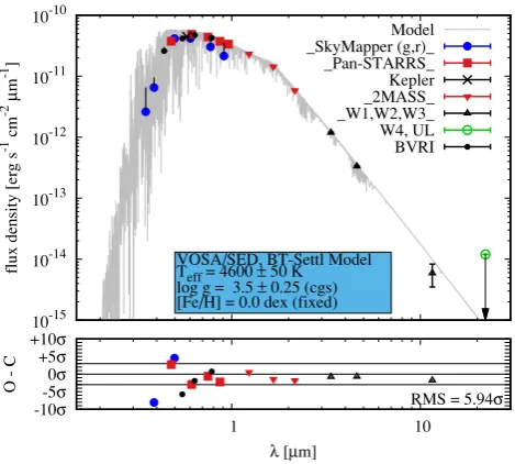
we compiled all available observed archive (reddened) broad-band photometric measurements (see Table 2) for our target and carried out a spectral energy distribution (SED) analysis. We used the Virtual Observatory SED Analysis (VOSA7_{v5.1) tool (Bayo}

et al.2008) for this purpose. VOSA derives stellar properties using theoretical atmosphere models from which synthetic photometry is calculated to fit the observed stellar magnitudes in various pass-bands. We considered the BT–Settl atmosphere model (Allard, Homeier & Freytag2012) for which grid models exist for a large range in the three main atmospheric parameters.

7_{http://svo2.cab.inta-csic.es/theory/vosa}

Table 2. Stellar parameters of EPIC 212737443. We derived the Johnson– Cousins (BJ,VJ) and Kron–Cousins (RC,IC) magnitudes from the precise Pan-STARRS1gP1,rP1,iP1magnitudes as a weighted mean using the linear

transformation equations from Tonry et al. (2012) and Kostov & Bonev (2018). The derived magnitudes, however, were not included in the SED modelling. For all considered models, we find that the SkyMapperu,v

andi,zflux densities are systematically underestimated when compared to the model-based flux densities. We indicate those points with the vertical lines in Fig.7. The acclaimed precision in those pass-bands seems too high and the associated errors are likely much larger in reality. We have therefore excluded the SkyMapperu,v,i,zdata and found models with a significantly smallerχ2

ν on the order ofχν230. Wehighlightdata that were included

in the SED modelling.

Parameter Value Source

Astrometry

αJ2000RA (hh:mm:ss) 13:36:53.21 GaiaDR2

δJ2000Dec. (dd:mm:ss) −07:19:05.32 GaiaDR2

π(mas) 2.95±0.04 GaiaDR2

Photometry

u(mag, 3490 Å) 17.731±0.029 SkyMapper

v(mag, 3840 Å) 17.324±0.055 SkyMapper g(mag, 5100 Å) 15.113±0.005 SkyMapper r(mag, 6170 Å) 14.494±0.010 SkyMapper i(mag, 7790 Å) 14.084±0.003 SkyMapper

z(mag, 9160 Å) 13.940±0.016 SkyMapper

gP1(mag, 4866 Å) 15.2645±0.0025 Pan-STARRS1

rP1(mag, 6215 Å) 14.4375±0.0039 Pan-STARRS1

iP1(mag, 7545 Å) 14.1158±0.0040 Pan-STARRS1

zP1(mag, 8679 Å) 13.9720±0.0009 Pan-STARRS1

yP1(mag, 9633 Å) 13.8671±0.0027 Pan-STARRS1

G(mag) 14.481±0.001 GaiaDR2

GBP(mag) 15.087±0.003 GaiaDR2

GRP(mag) 13.743±0.004 GaiaDR2

J(mag, 1.26μm) 12.824±0.026 2MASS

H(mag, 1.60μm) 12.239±0.026 2MASS

Ks(mag, 2.22μm) 12.160±0.024 2MASS W1 (mag, 3.4μm) 12.093±0.023 AllWISE W2 (mag, 4.6μm) 12.149±0.023 AllWISE W3 (mag, 12.0μm) 12.609±0.442 AllWISE W4 (mag, 22.0μm) 9.074 (see text) AllWISE

Derived photometry

BJ(mag) 15.963±0.0034 This work

VJ(mag) 14.836±0.013 This work

RC(mag) 14.191±0.016 This work

IC(mag) 13.626±0.017 This work

Kp(mag) 14.46±0.13 This work

The effect of interstellar extinction was accounted for in the SED modelling by adopting the mean extinction law for interstellar dust

RV = 3.1± 0.1 as described by Fitzpatrick (1999). The colour

excess E(B − V) was obtained from the Bayestar158 _sight-line

3D dust map provided by Green et al. (2015) using the distance inferred fromGaiaDR2. We determinedE(B−V)=0.01+₋00..0201.

The resulting extinction was found to be in the range AV ∈ [0,

0.083]. This reddening is somewhat consistent with the value (0.04) found by Huber et al. (2017) and is concordant with the

K2 Campaign 6 field of view being outside the galactic plane,

8_{http://argonaut.skymaps.info/}

where reddening in general is expected to be small. The five model parameters wereTeff, logg, [Fe/H],AV, andMd, where the latter

parameter is a flux density proportionality factor. TheGaiaparallax distance to EPIC 212737443 was included in the SED analysis to obtain an estimate of the stellar radius from the derived total flux estimate. For EPIC 212737443, the 2MASSJHKsphotometry

in particular is of great value to constrain Teff due to probing

different slopes on the SED. We chose to discard theu, v, i, z SkyMapper measurements since they consistently underestimate the theoretical flux densities. They are discrepant at a>10σ level. Including SkyMapper (u,v,i,z) data produced fits withχ2

νtypically larger than 200. Also, theGaiameasurements were not included as the three spectral windows are too broad. Derived photometric pass-bands including theKeplerand the AllWISEW4 (upper limit magnitude only) magnitudes were also not included in the final SED analysis. Table2indicates which data were used in the SED analysis.

Initially, we let all model parameters float freely. Based on the BT–Settl model, we found values of Teff=(4600±50) K,

logg=(4.5±0.35) cgs, and [Fe/H]=(−1.0±0.25) dex. The re-duced chi-squaredχ2

ν was found to be 34.3 for (13–5) degrees of freedom. As a rule of thumb (C. Rodriges, private communication) good SED models have 10 < χ2

ν < 50. Errors were found from a Monte Carlo bootstrapping method and are mainly limited by the grid mesh for a given parameter. The surface gravity is consistent with the (J − Ks, RPMJ) measurement for our star (see earlier

section). The most accurate parameter from an SED model is the

Teff. However, in our case an uncertainty of 50 K is judged to be

too optimistic. The surface gravity and metallicity are in general poorly constrained from broad-band photometry and are therefore the least accurate quantities. In our second experiment, we fixed the metallicity to [Fe/H] = 0.0 dex since a [Fe/H] = −1.0 dex is rarely found for stars in the solar neighbourhood. Fixing the metallicity to a solar value is empirically justified following the work by Guo et al. (2017). The authors found a mean metallicity of [M/H]mean=(−0.045±0.009) dex from a sample of 800

Kepler target stars. This value is significantly (3.8σ) larger than the metallicity estimate from the first SED experiment for a freely floating metallicity. Based on the BT–Settl model, we found values ofTeff=(4600±50) K, logg=(3.5±0.25) cgs for a fixed [Fe/H]

=0.0 dex. The reduced chi-squaredχ2

ν was found to be 50.9 for (13–4) degrees of freedom. While the effective temperature has not changed (with a possibly too optimistic uncertainty); the surface gravity changed by 2.3σ between the two runs.

From the distance, total flux, and effective temperature, as obtained from the second experiment, the stellar radius is found to be R=(0.660±0.019) R. From the surface gravity and the radius estimate, we find an unreliablestellar mass ofM= (0.050±0.029) M and should be ignored. The SED produced from VOSA is shown in Fig7. In a final attempt, we tried to estimate the stellar metallicity from considering various evolutionary tracks (Siess, Dufour & Forestini2000) in a colour–absolute magnitude diagram. We found the uncertainties in the absolute magnitude to be too high in order to constrain the metallicity for this star. For the remainder of this work, we therefore adopt a metallicity estimate of [Fe/H] = 0.0 dex as suggested empirically by Guo et al. (2017).

3.7 Stellar mass and radius – I

To obtain estimates for the stellar mass and radius, we used the method outlined in (Da Silva et al.2006) made available via the

10-15

10-14

10-13

10-12

10-11

10-10

flux density [erg s

-1 cm -2μ

m

-1]

Model _SkyMapper (g,r)_ _Pan-STARRS_ Kepler _2MASS_ _W1,W2,W3_ W4, UL BVRI

VOSA/SED, BT-Settl Model

T_eff = 4600 ± 50 K

log g = 3.5 ± 0.25 (cgs)

[Fe/H] = 0.0 dex (fixed)

-10σ

-5σ

0σ

+5σ

+10σ

1 10

O - C

λ [μm]

RMS = 5.94σ

Figure 7. Spectral energy distribution (log (Fλ)) as obtained from VOSA.

The SED is obtained from the BT–Settl atmosphere model. Filter character-istics were taken from the Spanish Virtual Observatory (SVO) filter profile service:http://ivoa.net/documents/Notes/SVOFPS/index.html. The reduced

χν2 was found to be 50.93. Data points are de-reddened. For some data

points, the error bar is smaller than the symbol size. The horizontal lines in the residual plot indicate±3σlevels.See electronic version for colours.

PARAM9 _{(v 1.3) web interface service. Stellar parameters are}

interpolated from stellar isochrones constrained by the bolometric luminosity and effective temperature. The luminosity is determined from Gaia DR2 parallax and the extinction-corrected V-band magnitude that we calculated from JHKs photometry using the

method in Huang et al. (2015). We used the previously (second SED experiment) determined values ofTeff, [Fe/H]=0.0, andmV=

(14.836±0.013) along withπ =(2.95±0.04) mas as input values, and found M=(0.713±0.012) M, R=(0.658±0.008) R, logg=(4.633±0.015) cgs. The radius estimate is in excellent agreement (0.1σ level) with the radius estimate obtained from the second SED run.

3.8 Stellar mass and radius – II

To produce a final set of parameters, we used theISOCHRONES (Morton2015a)PYTHON interface to the MIST stellar evolution models (Dotter 2016). The parameters are calculated with the 2MASSJHKsband photometry andGaiaDR2 parallax

measure-ments. Initially, we used Gaussian priors onTeff and loggbased

on our results from Section 3.5, and posterior samples via the MULTINEST algorithm (Feroz et al. 2013). We found that Teff=

(4684±79) K, logg=(4.622±0.024) cgs, [Fe/H]= −(0.137± 0.127) dex, M=(0.690±0.038) M,R=(0.673±0.024) R, and AV =0.150+₋00..186108mag. We then removed the priors on Teff

and logg to get another set of values using only the broad-band photometry and Gaia DR2 parallax. No change was seen between the outputs, except the metallicity that had a value of [F e/H]= −(0.180±0.124) dex in the second run. We also found that the mean stellar density ρ=3.190+₋00..256250 that is in

good agreement with the values derived in Section 3.2. We

9_{http://stev.oapd.inaf.it/cgi-bin/param 1.3}

Table 3. Adopted physical and atmospheric parameters for EPIC 212737443 usingISOCHRONES(Morton2015a).

Parameter Value Source

Teff(K) 4684±79 This work

logg(cgs) 4.622±0.024 This work

[Fe/H] (dex) −0.137±0.127 This work

R(R) 0.673±0.024 This work

M(M) 0.690±0.038 This work

Distance (pc) 347.449±12.014 This work AV(mag) 0.150+₋00..186108 This work

ρ(g cm−3) 3.190₋+0₀._.256₂₅₀ This work

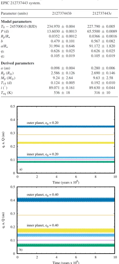
used this value of the mean density as a prior in the transit analysis (see Section 3.2). The final parameters are given in Table3. In addition, we added updated parameters for the two planets in Table4.

4 S TAT I S T I C A L VA L I DAT I O N

An assessment of the probability that the transits are astrophysical false positives was conducted using theVESPA software package (Morton 2015b). VESPA utilizes the Trilegal Galaxy model (Girardi et al. 2005) to determine the posterior probabilities for planetary scenarios and a set of false positive scenarios. The false positive scenarios taken into account include a blended background eclipsing binary, a hierarchical triple system, and the star is an eclipsing binary. All these scenarios are simulated by modelling the host star and its background, which are then compared to the observed phase-folded light curve. VESPA uses the broad-band photometric data, spectroscopic priors, and the contrast curves described in Section 2 as input. Additionally, we use the physical parameters of the planets and host star as calculated in Section 3, and constraints on the secondary eclipse depth and maximum exclusion radii. We use the criterion that if the FPP is<1 per cent then the planet is considered validated (Montet et al.2015; Crossfield et al. 2016). For this system,VESPA returned FPP values of 4.79×10−5

and 1.15×10−8_{for planetsbandc, respectively. Candidates in}

multitransiting systems are much more likely to be planets than those in single transit systems (Lissauer et al.2012), whichVESPA does not take into account. It was estimated that candidates in systems with two transits are 25 times more likely to be planets, thus the true FPPs are likely even lower than the above estimates fromVESPA. We therefore consider this to be a validated system of two planets.

5 DY N A M I C A L S TA B I L I T Y

We carried out a dynamical stability analysis based on the proba-bilistic mass–radius relation of Wolfgang, Rogers & Ford (2016). Using the mass–radius relation, the planet masses were found to be (9.24±2.64)M_⊕and (9.63±2.58)M_⊕, forbandc, respectively. We employed theMERCURY6 orbit integration package (Chambers 1999) and utilized the mixed-variable symplectic algorithm with a constant time stepping of 1/10 d. We integrated several initial orbital configurations aiming at investigating the orbital stability as function of the initial phase and eccentricity. Co-planar orbits were considered. The initial semimajor axis values were set to the derived values obtained from the best-fitting model. Several orbital configurations were integrated for 105_{yr. Long-term integration}

Table 4. Final best-fitting and derived parameters for the two planets in the EPIC 212737443 system.

Parameter (units) 212737443b 212737443c

Model parameters

T0−2457000.0 (BJD) 234.970±0.004 227.790±0.005

P(d) 13.6030±0.0013 65.5500±0.0089

Rp/R 0.0352±0.0012 0.0366±0.0016

b 0.479±0.101 0.567±0.082

a/R 31.994±0.646 91.172±1.820

q1 0.626±0.025 0.626±0.025

q2 0.105±0.019 0.105±0.019

Derived parameters

a(au) 0.098±0.004 0.280±0.006

Rp(R⊕) 2.586±0.126 2.690±0.146

Mp(M⊕) 9.24±2.64 9.63±2.58

T14(d) 0.124±0.005 0.192±0.010

i(◦) 89.071±0.161 89.630±0.044

Teq(K) 536±18 316±10

0 0.1 0.2 0.3 0.4 0.5

0 2 4 6 8 10

q, a, Q (au)

Time (years x 106) inner planet, e₀ = 0.20

outer planet, e₀ = 0.20

a)

0 0.1 0.2 0.3 0.4 0.5

0 2 4 6 8 10

q, a, Q (au)

Time (years x 106) inner planet, e₀ = 0.40

outer planet, e₀ = 0.40

b)

Figure 8. Time evolution of pericentre distance (q), semimajor axis (a), and apocentre distance (Q) for the two transiting planets considering a 107_yr

integration. Results for two initial eccentricities are shown.See electronic version for colours.

spanned a time period of 107_{yr. After integration, the relative energy}

change was at the order of a few part in 109_{. The results are shown}

in Figs8(a)–(c). We chose to display the time evolution of the pericentre distance (q=a(1−e)), semimajor axis (a), and apocentre distance (Q=a(1+e)) for various eccentricities of the two planets providing information on the eccentricity variation. System stability

for the two-planet system is demonstrated for low to moderate initial eccentricities from 0.0 up to 0.40 for both planets. The system became unstable at eccentricities over 0.40, implying the onset of orbit crossing between the two planets, thus imposing a constraint on the eccentricities that are possible for each planet. For initial circular and near-circular orbits the mutual perturbations are small for the considered masses and the system stability is qualitatively guaranteed over the 107_{yr. Mutual gravitational perturbations seem}

small for the considered masses.

6 D I S C U S S I O N

In the context ofK2 exoplanets, planetchas the longest confirmed orbital period with two or more observed transits.10_{The HIP41378}

system is thought to contain three planets with orbital periods above 100 d (Vanderburg et al.2016b), but are yet to be precisely measured (Becker et al.2018; Berardo et al.2018).

Using the equationTeq=T∗(R∗/2a)1/2[f(1−AB)1/4] , and applying

f=1 (Koch et al.2010) with a bond albedo ofAB=0.3, we find

the equilibrium temperatures of planetsbandcto be 536±18 K and 316±9 K, respectively, making them both temperate planets. Again, planetcstands out as the coolest planet found around a star earlier than an M-type star within theK2 mission.11

Since planetc only exhibits two transits, there is a non-zero probability that the transits are from two distant planets as opposed to being from a single body (Benneke et al.2017). In Section 3.2, we showed that when the two transits are taken individually, they have near-identical transit depths and transit durations. In addition, we demonstrated that if the transits are from two separate objects with circular, equatorial orbits, they would have minimum periods of 68.6 and 80.2 d with transit durations longer than what was observed. We carried out an additional investigation to determine the transit durations if these orbits are eccentric with non-zero impact parameters. We found that the theoretical durations become more consistent with the observed durations for values of b between 0.45 and 0.6, eccentricities between e=0.25 and e =0.4. If the orbits are moved further away from each other, stable orbits with a high eccentricity that could replicate the observed data become more likely. Therefore, we acknowledge the possibility that the two transits spaced 65 d apart could be from two different bodies. But based on our analysis, a two-planet system with planetchaving a period of 65 d seems the simpler explanation for the observations. The current ephemeris of planetccould be used to predict when future transits would happen, and targeted observations could be carried out at a specific time with a telescope such as theSpitzer Space Telescopeor CHEOPS. The observation of a third transit at a predicted time would confirm if the two transits seen in our data belong to the same object.

We computed the mutual Hill radius (RH) between the two

planets using the methods in Weiss et al. (2018). As the mutual Hill radius is dependent on the planet masses, we used both the empirical relationship in Weiss & Marcy (2014) as well as the relationship in Wolfgang et al. (2016), and foundRH =33.1

and 36.2, respectively. Similarly, we found the values ofRHfor

all adjacent pairs of planets validated throughout theK2 campaign. The distribution ofRHwas consistent between the values of 10

and 30 (with the Weiss & Marcy relation), with only two adjacent pairs having values below 10. Of 81 pairs, only 12 adjacent pairs

10_{https://exoplanetarchive.ipac.caltech.edu/cgi-bin/TblView/nph-tblView} 11_{http://www.openexoplanetcatalogue.com/systems/}

have mutual Hill radii higher than that of the EPIC 212737443 system. All but one of the planet pairs contain either an ultrashort-period planet (P < 1 d), a pair of super-Earth-type planets or two planets with radii differing by more than 1R_⊕. EPIC 212737443 is the onlyK2 system withRH>35 including two planets with

near-equal size. Weiss et al. (2018) concluded that there is a correlation between the radii of planets and the spacing between adjacent pairs. The implication of this correlation is that systems with similarly sized planets could potentially be direct remnants from the planet formation phase (Millholland, Wang & Laughlin2017). In terms of Hill radii, there is a lot of space in this system for a third planet to trace an orbit between planetsbandc. Either a potential third planet is too small to be detected given the noise floor, could be a non-transiting planet (inclined orbit), or it could have been ejected from the system as a result of a past encounter event. We usedMERCURY6 once again to place an 9M_⊕mass planet on a circular orbit between planetsbandcto test the system stability. The simulation resulted in a stable configuration over 107_{yr, adding to the likelihood of a third}

planet. However, the sample of Kepler systems studied in Weiss et al. (2018) and our analysis ofK2 systems show that a majority of compact multiplanet systems contain planets of similar sizes. This means it is much more likely that another sub-Neptune sized planet lies between the validated planets, instead of a small planet that could not be detected. The implication here is that if a third planet exists, it is most likely to be non-transiting or have been ejected. Future follow-up observations will certainly be needed. However, the main issue for such observations is the faint nature of this star requiring a large aperture telescope.

7 S U M M A RY

In conclusion, we used a light curve from theK2 mission along with high-resolution imaging to characterize and confirm a system of two planets around EPIC 212737443. Planet bhas an orbital period of (13.603±0.0013) d of and a radius of (2.580±0.084)R⊕, while planetc has a period of (65.550±0.0089) d and a radius of 2.660±0.128R_⊕. The radii of the two planets puts them firmly within the size regime of sub-Neptune-type planets. Their sizes imply that the planets are most likely gaseous, or contain significant amounts of volatiles such as water. The large mutual Hill radius of the system opens up the possibility for an additional planet of near-equal sizes between planetsband c. The study of systems with large values forRH, such as EPIC 212737443, would add to the

ongoing investigations of multiplanet systems to learn more about how planets are arranged and the implications for their formation histories.

AC K N OW L E D G E M E N T S

The authors would like to thank the anonymous referee for im-proving this research paper. MH, TCH, JHL, and CTKL would like to thank the organizers of the 2018 February Recontres du Vietnam conference where this work was originally initiated. This paper includes data collected by the Kepler/K2 mission. Funding for theKeplermission is provided by the NASA Science Mission directorate. This publication uses data products from the (1) WISE – Wide-field Infrared Survey Explorer, which is a joint project of the University of California, Los Angeles, and the Jet Propulsion Laboratory/California Institute of Technology, funded by the National Aeronautics and Space Administration; (2) SkyMapper – the National Facility Capability for SkyMapper has been funded through ARC LIEF grant LE130100104 from

the Australian Research Council; (3) Gaia – This work has used data from the European Space Agency (ESA) missionGaia

(https://www.cosmos.esa.int/gaia), processed by the Gaia Data Processing and Analysis Consortium (DPAC, https://www.cosm os.esa.int/web/gaia/dpac/consortium). Funding for the DPAC has been provided by national institutions, in particular the institutions participating in theGaiaMultilateral Agreement; (4) Pan-STARRS – https://panstarrs.stsci.edu/. This publication uses (1) VOSA, developed under the Spanish Virtual Observatory project supported from the Spanish MICINN through grant AyA2011-24052; (2) the VizieR catalogue access tool, CDS, Strasbourg, France. The original description of the VizieR service was published in A&AS 143, 23; (3) DSS2 (http://archive.eso.org/dss/dss). TCH would like to acknowledge a fruitful discussion with Dr. Eric Mamajek and Dr. Andrew Mann related to atmospheric properties of stars.

R E F E R E N C E S

Allard F., Homeier D., Freytag B., 2012,Phil. Trans. R. Soc. A, 370, 2765 Bailer-Jones C. A. L., 2015,PASP, 127, 994

Barros S. C. C., Demangeon O., Deleuil M., 2016,A&A, 594, A100 Bayo A., Rodrigo C., Barrado Y Navascu´es D., Solano E., Guti´errez R.,

Morales-Calder´on M., Allard F., 2008,A&A, 492, 277 Becker J. C. et al., 2018, AJ, 156, 81

Benneke B. et al., 2017,ApJ, 834, 187

Bensby T., Feltzing S., Lundstr¨om I., 2003,A&A, 410, 527 Berardo D. et al., 2018, AJ, 157, 51

Borucki W. J. et al., 2010,Science, 327, 977 Chambers J. E., 1999,MNRAS, 304, 793

Chambers K. C. et al., 2016,https://arxiv.org/abs/1612.05560 Claret A., Hauschildt P. H., Witte S., 2012, A&A, 546, A14 Crossfield I. J. M. et al., 2016,ApJS, 226, 7

da Silva L. et al., 2006,A&A, 458, 609

Dehnan W., Binney James J., 1998,MNRAS, 298, 387 Dotter A., 2016,ApJS, 222, 11

Dressing C. D., Newton E. R., Schlieder J. E., Charbonneau D., Knutson H. A., Vanderburg A., Sinukoff E., 2017,ApJ, 836, 167

Evans D. F. et al., 2016, A&A, 589, A58 Evans D. F. et al., 2018, A&A, 610, A20

Feroz F., Hobson M. P., Cameron E., Pettitt A. N., 2013, preprint (arXiv: 1306.2144)

Fitzpatrick E. L., 1999,PASP, 111, 63

Foreman-Mackey D., Hogg D. W., Lang D., Goodman J., 2013,PASP, 125, 306

Gaia Collaboration, 2018b,A&A, 616, A10 Giles H. A. C. et al., 2018, A&A, 615, L13

Girardi L., Groenewegen M. A. T., Hatziminaoglou E., da Costa L., 2005, A&A, 436, 895

Gould A., Morgan C. W., 2003,ApJ, 585, 1056 Green G. M. et al., 2015,ApJ, 810, 25

Guo X., Johnson J. A., Mann A. W., Kraus A. L., Curtis J. L., Latham D. W., 2017,ApJ, 838, 25

Herter T. L. et al., 2008, in McLean I. S. , Casali M. M., eds, Proc. SPIE Conf. Ser. Vol. 7014, Ground-based and Airborne Instrumentation for Astronomy II. SPIE, Bellingham, p. 70140X

Horch E. P., Howell S. B., Everett M. E., Ciardi D. R., 2012,AJ, 144, 165 Horch E. P., Veillette D. R., Baena Gall´e R., Shah S. C., O’Rielly G. V., van

Altena W. F., 2009,AJ, 137, 5057 Horch E. P. et al., 2017,AJ, 153, 212

Howell S. B., Everett M. E., Sherry W., Horch E., Ciardi D. R., 2011,AJ, 142, 19

Howell S. B. et al., 2014,PASP, 126, 398

Huang C. X., Penev K., Hartman J. D., Bakos G. ´A., Bhatti W., Domsa I., de Val-Borro M., 2015,MNRAS, 454, 4159

Huber D. et al., 2014,ApJS, 211, 2 Huber D. et al., 2016,ApJS, 224, 2

Husser T.-O., Wende-von Berg S., Dreizler S., Homeier D., Reiners A., Barman T., Hauschildt P. H., 2013, A&A, 553, A6

Kipping D. M., 2013,MNRAS, 435, 2152 Koch D. G. et al., 2010,ApJ, 713, L131 Kostov A., Bonev T., 2018, Bulg. Astron. J., 28, 3 Kov´acs G., Zucker S., Mazeh T., 2002,A&A, 391, 369 Kreidberg L., 2015,PASP, 127, 1161

Kupfer T.et al., 2018, MNRAS, 480, 302 Lissauer J. J. et al., 2012,ApJ, 750, 112 Luri X. et al., 2018, A&A, 616, A9 Mandel K., Agol E., 2002,ApJ, 580, L171 Mayo A. W. et al., 2018b,AJ, 155, 136

Millholland S., Wang S., Laughlin G., 2017, ApJ, 849, L33 Montet B. T. et al., 2015,ApJ, 809, 25

Mortier A. et al., 2018,MNRAS, 481, 1839

Morton T. D., 2015a, Astrophysics Source Code Library, record ascl:1503.010

Morton T. D., 2015b, Astrophysics Source Code Library, record ascl:1503.011

Ofir A., 2014,A&A, 561, A138

Pope B. J. S., Parviainen H., Aigrain S., 2016,MNRAS, 461, 3399 Reddy B. E., Lambert D. L., Allende Prieto C., 2006,MNRAS, 367,

1329

Scott N. J., Howell S. B., Horch E. P., 2016, in Malbet F., Creech-Eakman M. J., Tuthill P. G., eds, Proc. SPIE Conf. Ser. Vol. 9907, Optical and Infrared Interferometry and Imaging V. SPIE, Bellingham

Sharma S., Bland-Hawthorn J., Johnston K. V., Binney J., 2011, ApJ, 730, 3

Siess L., Dufour E., Forestini M., 2000, A&A, 358, 593 Skottfelt J. et al., 2015, A&A, 574, A54

Skrutskie M. F. et al., 2006,AJ, 131, 1163

Soubiran C., Bienaym O., Siebert A., 2003,A&A, 398, 141 Tonry J. L. et al., 2012,ApJ, 750, 99

Vanderburg A., Johnson J. A., 2014,PASP, 126, 948 Vanderburg A. et al., 2016,ApJ, 827, L10

Weiss L. M., Marcy G. W., 2014,ApJ, 783, L6 Weiss L. M. et al., 2018,AJ, 155, 48 Wisdom. J., 1980,AJ, 85, 1122

Wolf C. et al., 2018,Publ. Astron. Soc. Aust., 35, 10 Wolfgang A., Rogers L. A., Ford E. B., 2016,ApJ, 825, 19 Wright E. L. et al., 2010,AJ, 140, 1868

This paper has been typeset from a TEX/LA_{TEX file prepared by the author.}