ECE-320 Lab 3: Utilizing a dsPIC30F6015 to model a DC motor and a wheel

1

ECE-320 Lab 3: Utilizing a dsPIC30F6015 to model a DC motor and a wheel

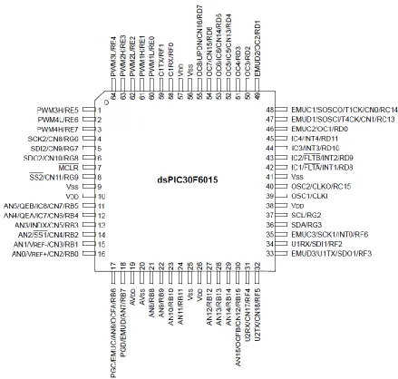
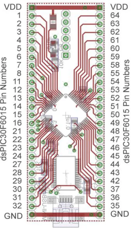
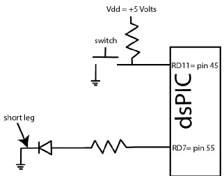
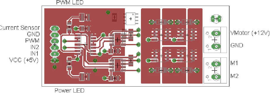
Overview: In this lab we will utilize the dsPIC30F6015 to model a DC motor that is used to control the speed of a wheel. Most of the initial code will be given to you (see the class website), and you will have to modify the code as you go on. One of the things you will discover is that you often need to be aware of limitations of both hardware and software when you try to implement a controller. The dsPIC30F6015 has been mounted on a carrier board that allows us to communicate with a terminal (your laptop) via a USB cable. In what follows you will need to make reference to the pin out of the dsPIC30F6015 (shown in Figure 1) and the corresponding pins on the carrier (shown in Figure 2)

2

Figure 2. dsPIC30F6015 carrier. Note that the pin numbers are not consecutive.

Part A (Copying the initial files)

3

Part B (Putting it all together)

Now we are ready to start. Note that at some point in the following process you may need to let the system download firmware. Be sure you have selected the correct device (or it will do this twice). Start MPLAB X IDE (not IPE)

Select File, then New Project (the screen should default to Mocrochip Embedded and Standalone Project)

Click on Next

In the Select Device section, select the following: Family: 16-bit DSCs (dsPIC30)

Device: dsPIC30F6015

Click on Next

In the Select Tool section, select PICkit3

Click on Next

In the Select Compiler section, select XC16

Click on Next

In the Select Project Name and Folder section, choose a name and project location Click on Finish

Make sure the file model_wheel.c is in the Project folder. Right click on Source Files, then on Add

Existing Item, then select model_wheel.c

4 You should build (compile) the existing program, download it to the dsPIC, and run it. You should see a sequence of numbers on your screen (the secure CRT screen). These correspond to sample times. If you see the following message

You are trying to change protected boot and secure memory. In order to do this you must select the "Boot, Secure and General Segments" option on the debug tool Secure Segment properties page.

Failed to program device

Then

 Right Click on the Project Name and select Properties

 Under Categories in the left panel, click on PICkit3

 Under Option categories at the top, select Secure Segment

 On the right select Boot, Secure, and General Segments

 Then select ok at the bottom.

Your program should now compile.

Part C: Reading in the sensor transducer

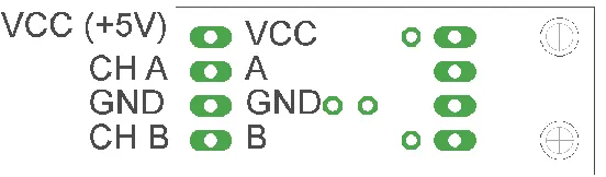
In order to determine how fast the wheel is spinning, we will need to use the QEI interface. The sensor is connected to the center of the wheel, and the other end of the sensor plugs into the breadboard. The pins for the interface are shown in Figure 3. You need to connect this interface to +5 volts (red ), ground (blue), and the QEA Channel A input (pin 12), and the QEA Channel B input (pin 11).

5

Part D (Reading in an A/D value)

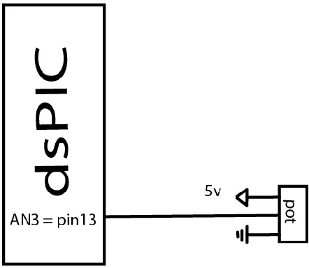
Now we want to be able to connect a potentiometer as shown in Figure 4 so we can have a variable reference. The software is currently set up for A/D input on AN3/RB3 (pin 13). You will need to do the following things:

 Connect the potentiometer as shown below

 Set the appropriate TRIS bits for an input signal

Note that this is the same set-up as was used in the previous lab.

Figure 4. Connecting the potentiometer

Part E: Connecting the shut off switch.

6

Figure 5. Setting up the external interrupt triggered shut off switch.

Part F: Connecting the power entry

Plug in both the 5 volt (green) and 12 volt (red) power supplies, as shown in Figure 6. Do not turn on the supplies yet (the LEDs should be off) .

7

Part G: Connecting the H bridge

Plug in the H-bridge, shown in Figure 7. You are going to need access to the different pins, so be sure it is located in a place you can easily get wires to.

Figure 7. H Bridge connections

Starting on the left, connect the ground and +5 volt supplies. Next, connect IN1 to RE6 (pin 2) and IN2 to RE7 (pin 3). (Note that if the motor speed is negative you need to reverse these connections.) Finally connect PWM to PWM 3 high (pin 1).

Starting on the right, connect (with the twisted wires) the 12 volt power from the power entry module to the 12 volt input. Be sure to connect ground to ground and +12 to +12. Next, connect M1 and M2 (using the twisted wires from the wheel) to the motor input.

At this point all of your wiring should be done. You should check it over before you go on.

Two important things to keep in mind as you do the remainder of this lab:

 Use your shut off switch to shut off the motor/stop the wheel. This actually stops the outputs, and puts the program in an infinite loop. You need to separately stop the program.

 You will then need to select the MPLAB stop button to stop the program (read square with white square inside, see next page.)

8

For this lab, it is probably much easier to use the debugging features in MPLABX

Click here to compile and download to PIC

Click here to pause Click here to exit (stop)

Click here to reset, this will stop the motor and

9 At this point we should be sure everything is working. Be sure the 5 volt supply is on (the green light should be on) and the 12 volt supply is off (the red light should be off). Compile the program and open SecureCRT so you can read the program output. When the program starts to run, the output to the screen is the current time, the value read from the pot, the dutycycle, and the speed of the wheel in radians/sec.

If you have done everything correctly, the LED should light, the reference signal (from the pot) should go from 0 to 1023, and the dutycycle should go from 0 to 14600. If you push the shutoff switch the program should stop and the LED should shut off. Be sure all of these parts are working before you go on. At the end of this step, be sure the pot is reading 0 and the dutycycle is at 0.

PART H: Determining initial scaling

Now we will start to determine some of our parameters to model the motor. Turn on the power to the motor (the red LED should turn on).

With the system at rest start the program and slowly turn the pot so the motor is spinning. The motor will not start for low input values so don’t be alarmed if nothing happens at first. Continue to turn the pot slowly until the motor starts to spin the wheel. Turn the pot so the motor is spinning at less than or equal to 30 rad/sec. If the speed of the wheel is negative reverse the polarity of the power wires to the motor. Let the motor come to a reasonably steady value (it will likely keep getting faster). Wait until the motor speed is fairly constant and the input reading from the pot is also fairly constant. Record the reading from the pot and the speed of the motor. Do this for three different positions of the pot where the steady state speed is less than 80 rad/sec. (Note that it is likely to be easiest to use the session log file than look at the screen output.) Stop the wheel by using your shut off switch!

We now want to determine the proportionality constant between the A/D value read from the pot and the motor speed in rad/sec. That is, we want to convert from the A/D value read from the pot to the speed of the wheel. Compute the three scaling factors and average them (mine was between approximately 0.15 and 0.23).

Change the parameter AD_scale (in your code) to this value. Run the system again at various input values. It may take a while for the system to reach steady state, and to read lower speeds like 30 rad/sec you may have to start at a higher speed and work your way down to the desired speed. Compare your reference input to the actual output. They should be fairly close for some speeds but they will not be exact. For other speeds they may be off by a significant amount. This is open loop control.

Part I: Belt Slippage

10 simple way to try to account for this is to monitor the changes in speed from one time instance to the next, and make sure the speed does not change by too much.

In the file model_wheel.c you need to:

 Define a constant at the top of the file MAX_DELTA_SPEED and set this value equal to 3.0

(this is somewhat arbitrary, it depends on how fast your system can move)

 Declare a double in the main routine named last_speed;

 Before the main while loop, set last_speed = 0.0;

 Within the main while loop, modify the code so it looks like the following:

speed = ((double)((r2-r1)*720+(p2-p1)))*speed_scale; // already in the code speed = min(speed, last_speed+MAX_DELTA_SPEED);

speed = max(speed, last_speed-MAX_DELATA_SPEED); speed = max(speed, 0.0);

last_speed = speed;

This should limit the spikes if the belt slips. We do loose some accuracy doing this, but this is better than reading in one of the erroneous speed signals and trying to react to it.

For the remainder of this lab we will be making a model of the plant, including some of the

nonlinearities of the DC motor. As you will see, this is still not an exact model. However, we will use this model in subsequent labs so try to do as well as you can.

PART J: Modeling the plant as a first order system

A simple mathematical model of our plant in the time domain is _p( )s a

G K

s 

 . Assuming a zero order

hold we will get the discrete-time model ( ) 1 aT

p aT

K e B

z

a z e z b

G



 

 

  . Note that we really only care about the discrete-time parameters B and b. If the input is then a step of amplitude R, we can write the output

as ( ) 1 ( ) C 1 ( )

1

n n

RB

y n b u n b u n

b   

 _  _  _  _

 . Since we know R and will determine b and C from the step response we can finally determine B as B C(1 b)

R 

 .

In the program model_wheel.c comment out the reference input coming from the pot and set the value of R to be 50 rad/sec. We are doing this so we have a fixed amplitude step input. Your code should look something like the following:

11 R = 50.0;

Next you need to go to SecureCRT and prepare to log the step response. The Matlab code we will use assumes the name of the file is Step_Response_50. Be sure to put this log file in a folder you can find (a good idea is in the current project file.) Note that if you try this multiple times you need to toggle the log

session choice. You toggle it once to start, and once to save the file. Each time you want a step response

you should do this (otherwise it saves everything).

Now we are ready to measure the step response of the system. Turn on the power to the board and the motor (both red and green LED’s should be lit) and compile the program. Once it starts let it run until steady state, but no longer than 15 seconds before you use your shutoff switch.

Now run the Matlab program wheel_match.m and adjust the parameters C and b until you get a reasonably good fit for the data (note that you may have to edit the data file to have the system start at time zero.) The value of Tmax indicates the last time you want to look at, so you can run the system for 15 seconds and then choose to just look at the first 10 seconds (or the first two seconds.) Note that this program initially assumes a delay of 3 samples (which we will get to). You may need to change this delay. It is most important to match the measured data for the first second or two and at the final value. Once you have a good overall fit you need to put a copy of your figure in your memo with a figure number and caption.

Now change the value of R to 75.0 and try this again. Record the data in a different file this time (like

Step_Response_75) and modify the code to use the new file. Note that you may have to change the

assumed delay to be something different than 3 (like maybe 4) to get the measured and estimated plots to start at the same place. Put a copy of this figure in your memo with a figure number and caption. In what follows use the average of the two values for b and B.

Part K: Including some nonlinearities in a Simulink model

Now we will start to make a Simulink model that includes some of the nonlinear effects of the system. The file DT_Openloop_driver.m will contain most of the parameters we need and it runs the Simulink file DT_Openloop.slx. As you can see, the Simulink file contains more than just the transfer function, it includes a few of the components we will use to model some of the nonlinearities of the system. At this point many of the parameters in the driver file are just dummies. The only nonlinear effect that has been included is a limitation on the control effort in the Control Effort Limit saturation block. Note that all of the units in the Simulink model are in rad/sec.

12 Now we will set the Speed Limit saturation block. Comment out the fixed value of R ( R=75.0) and use the pot as the input (uncomment R = (double)….). Turn off the motor power (the red LED) and be sure the board power (green LED) is on. Compile and run the system to be sure the reference signal is being read from the pot. Set the input to zero and stop the system. Now turn on the power to the motor, and run the system again. This time slowly turn the pot all the way on, and see how fast the motor can go. Only let the motor run for at most 15-20 seconds, record the maximum speed of the motor, and then turn the pot back down to zero before shutting off the motor. Set the Max_Speed variable equal to this maximum value.

As you have probably noticed, the motor does not start spinning until the input gets to a certain value, and then it stops spinning at a different value. This is hysteresis and we will try and model it next. With the input at zero, slowly increase the value of the input until the motor (wheel) just starts to turn and record the value of the input (in rad/sec.) Now decrease the input signal slowly until the motor (wheel) stops and record this input (in rad/sec). Go through this process a few times until you feel you are getting consistent results (you might want to average the results for turning on and turning off). The

Relay_On variable should be set to the value that makes the system start moving, and the Relay_Off

variable should be set to the value where the system stops moving.

PART L: Openloop control

13

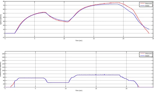
Figure 8. Bob’s result for the open loop system.

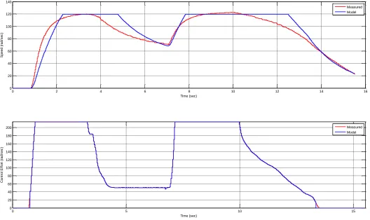
Next we want to run the openloop system again, but this time we want to make the control effort reach it’s saturation level. This means we need to turn the pot all the way on in a short period of time. You may get some spikes in your data if the belt is slipping. I ran my system for around 15 seconds and got the results shown in Figure 9. Note that the control effort has clearly reached saturation, and the model and real system do not match too well. Include a copy or this figure in your memo.

0 5 10 15 20 25

-10 0 10 20 30 40 50 60 70 80 Time (sec) S p e e d ( ra d /s e c ) Measured Model

0 5 10 15 20

14

Figure 9. Openloop response reaching control effort saturation.

Part M : Limiting slew rate

The last thing we want to model is limiting the slew rate of the motor, or how fast we allow the control effort to increase. This is something that does not happen with this system much, but it is likely to happen with different types of systems so we should go over it. We will need to modify both the

model_wheel.c code and the DT_Openloop_driver.m file.

In the file model_wheel.c you need to:

 Define a constant at the top of the file MAX_DELTA_U and set this value equal to 100

 Declare a double in the main routine named last_u;

 Before the main while loop, set last_u = 0.0;

 Within the main while loop, modify the code so it looks like the following: u = min(u, last_u+MAX_DELTA_u);

u = min(u, MAX_U); u = max(u,0.0); last_u = u;

0 2 4 6 8 10 12 14 16

0 20 40 60 80 100 120 140 Time (sec) S p e e d ( ra d /s e c ) Measured Model

0 5 10 15

15 In the file DT_Openloop_driver.m you need to set the value of MAX_DELAT_U (all of the scaling will be done for you.)

Rerun your system for a step input of 75 rad/second, and run DT_Openloop_driver.m to compare the model with your real system. They should be fairly close (except for the control effort at the beginning.) Include this plot in your memo.