Cancer Absolute Risk Projection with Incomplete Predictor Variables

(1)

University of Pennsylvania

ScholarlyCommons

Publicly Accessible Penn Dissertations

1-1-2015

Cancer Absolute Risk Projection with Incomplete

Predictor Variables

Lu Chen

University of Pennsylvania, [email protected]

Follow this and additional works at:http://repository.upenn.edu/edissertations Part of theBiostatistics Commons

This paper is posted at ScholarlyCommons.http://repository.upenn.edu/edissertations/1027 For more information, please [email protected].

Recommended Citation

Chen, Lu, "Cancer Absolute Risk Projection with Incomplete Predictor Variables" (2015).Publicly Accessible Penn Dissertations. 1027.

(2)

Cancer Absolute Risk Projection with Incomplete Predictor Variables

Abstract

A popular approach to projecting cancer absolute risk is to integrate a relative hazard function of predictors with hazard rates obtained from different sources, where the relative hazard function is often approximated by an odds ratio function. To assess added values of candidate risk predictors, it is very common that data for standard risk predictors is fully available from a frequency-matched case-control study, but that of candidate predictors is available only for a subset of cases and controls. In the first project, we developed statistical measures for quantifying predictive accuracy of cancer absolute risk prediction models, accommodating incomplete predictor variables. We particularly focused on a measure that is useful for evaluating efficiency of model-based cancer screening, the proportion of cases that can be captured by screening only people with high projected risk. In the second project, using a logistic regression model to describe the relationship between cancer status and risk predictors, we developed a novel semiparametric maximum likelihood approach that accommodates incomplete predictor data under rare disease approximation for the estimation of odds ratio parameters and the distribution of candidate predictors. Through theoretical and simulation studies, we showed that our estimator is consistent with an asymptotically normal distribution and has improved statistical efficiency. In the third project, we applied the statistical methods developed in the first two to evaluate the added values of percent mammographic density and breast cancer risk SNPs in breast cancer absolute risk projection. Our results showed that the two sets of predictors had similar added values and can lead to more efficient model-based screening for breast cancer. In the fourth project, we applied the semiparametric maximum likelihood method to a family-supplemented study design that we proposed to address survival bias in case-control genetic association studies.

Degree Type

Dissertation

Degree Name

Doctor of Philosophy (PhD)

Graduate Group

Epidemiology & Biostatistics

First Advisor

Jinbo Chen

Keywords

Absolute risk prediction, Breast cancer, Predictive accuracy, Semi-parametric maximum likelihood, Stratified case-control study, Two phase design

Subject Categories

(3)

CANCER ABSOLUTE RISK PROJECTION WITH INCOMPLETE PREDICTOR VARIABLES

Lu Chen

A DISSERTATION

in

Epidemiology and Biostatistics

Presented to the Faculties of the University of Pennsylvania

in

Partial Fulfillment of the Requirements for the

Degree of Doctor of Philosophy

2015

Supervisor of Dissertation

Jinbo Chen, Associate Professor of Biostatistics

Graduate Group Chairperson

John H. Holmes, Professor of Medical Informatics in Epidemiology

Dissertation Committee

Hongzhe Li, Professor of Biostatistics

Rebecca A. Hubbard, Associate Professor of Biostatistics

Andrea B. Troxel, Professor of Biostatistics

(4)

CANCER ABSOLUTE RISK PROJECTION WITH INCOMPLETE PREDICTOR

VARIABLES

c

COPYRIGHT

2015

Lu Chen

This work is licensed under the

Creative Commons Attribution

NonCommercial-ShareAlike 3.0

License

To view a copy of this license, visit

(5)

ACKNOWLEDGEMENT

I would like to thank my advisor and mentor, Dr. Jinbo Chen, for her guidance

thoughout my dissertation. She is patient, kind, encouraging, and always willing to

answer questions. She is also a great instructor who teaches enthusiastically and

sin-cerely. Without Dr. Chen, it would be impossible for me to complete this work. I

am grateful to Dr. Hongzhe Li for his support throughout the program. Dr. Li is my

committee chair who has been providing many insightful advices, and the instructor

of the course Probability, which was the first class I took in this department and the

stepping stone for me in this field. I would also like to thank my committee members

Dr. Rebecca Hubbard, Dr. Andrea Troxel, Dr. Emily Conant and Dr. Daniel

Heit-jan (my candidacy examination committee member) who provided numerous helpful

suggestions for my research. I further would like to thank all the faculty members

and staff in the Department of Biostatistics and Epidemiology. Their instruction,

kindness and considerateness have led me to learn and grow up. I also need to thank

the fellow students Jarcy, Daniel, Matthew, Jiwei, Emin and Vicky. We have spent

much time together to get though all the course work and qualifying examination.

Their love and help made me quickly accustomed to the academic environment and

life in University.

I would also like to thank my husband Xiao Ji for his love and support during the

dissertation. Grateful thanks to my best friend Christy Wang who helped me find

out the reason why I do research - to re-discover His creation and to re-search for His

(6)

ABSTRACT

CANCER ABSOLUTE RISK PROJECTION WITH INCOMPLETE PREDICTOR

VARIABLES

Lu Chen

Jinbo Chen

A popular approach to projecting cancer absolute risk is to integrate a relative hazard

function of predictors with hazard rates obtained from different sources, where the

relative hazard function is often approximated by an odds ratio function. To assess

added values of candidate risk predictors, it is very common that data for standard

risk predictors is fully available from a frequency-matched case-control study, but that

of candidate predictors is available only for a subset of cases and controls. In the first

project, we developed statistical measures for quantifying predictive accuracy of

can-cer absolute risk prediction models, accommodating incomplete predictor variables.

We particularly focused on a measure that is useful for evaluating efficiency of

model-based cancer screening, the proportion of cases that can be captured by screening

only people with high projected risk. In the second project, using a logistic

regres-sion model to describe the relationship between cancer status and risk predictors, we

developed a novel semiparametric maximum likelihood approach that accommodates

incomplete predictor data under rare disease approximation for the estimation of odds

ratio parameters and the distribution of candidate predictors. Through theoretical

and simulation studies, we showed that our estimator is consistent with an

asymptot-ically normal distribution and has improved statistical efficiency. In the third project,

(7)

values of percent mammographic density and breast cancer risk SNPs in breast

can-cer absolute risk projection. Our results showed that the two sets of predictors had

similar added values and can lead to more efficient model-based screening for breast

cancer. In the fourth project, we applied the semiparametric maximum likelihood

method to a family-supplemented study design that we proposed to address survival

(8)

LIST OF TABLES

TABLE 2.1 : Estimates of the OR Parameters for BCDDP. . . 24 TABLE 2.2 : Estimates of Predictive Accuracy Statistics for the BCRAT

and its Variants. . . 25 TABLE 2.3 : OR Estimates in Simulation Studies with 2 SNPs. . . 29 TABLE 2.4 : Estimates of Predictive Accuracy Statistics in Simulation

Stud-ies with 2 SNPs. . . 31 TABLE 2.5 : Estimates of Predictive Accuracy Statistics in Simulation

Stud-ies with 74 SNPs. . . 33

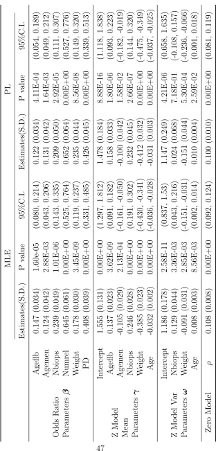
TABLE 3.1 : Estimates of Odd Ratio Parameters for the BCDDP Study. . 47

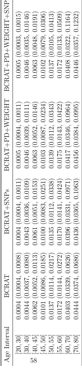
TABLE 4.1 : Estimates of Absolute Risk by Model: Mean (Median, 95% Range). . . 58 TABLE 4.2 : Proportion of Women with Absolute Risk Greater than

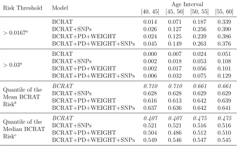
Cer-tain Risk Cutoff in Each Age Intervals by Model. . . 59 TABLE 4.3 : Estimates of Predictive Accuracy Statistic by Age Interval,

Cutoff and Model. . . 60 TABLE 4.4 : Mean Absolute Risk in Every Quintile by Model. . . 61

TABLE 5.1 : Estimated Type I Error Rates for Testing Association (nomi-nal level=0.5) When Deceased Cases were Na¨ıvely Ignored. . 81 TABLE 5.2 : Parameter Estimation under Different Models and Scenarios

for Genotyping Family Members of Deceased Cases. . . 82

TABLE B.1 : Estimates of Z model Parameters in Real Data Analysis. . . 107 TABLE B.2 : 74 SNPs from External Sources in Real Data Analysis. . . . 108 TABLE B.3 : Estimates of Predictive Accuracy Statistics with Absolute Risk

Cutoff in Real Data Analysis. . . 110 TABLE B.4 : Estimates of Z Model Parameters in Simulation with 2 SNPs

(Moderate Assocation). . . 111 TABLE B.5 : Estimates of Predictive Accuracy Statistics with Absolute Risk

Cutoff in Simulation Studies with 2 SNPs. . . 112 TABLE B.6 : Estimates of Z Model Parameters in Simulation with 74 SNPs. 113 TABLE B.7 : Estimates of 74 SNPs Odds Ratio Parameters in Simulation. 114 TABLE B.8 : Estimates of Parameters under Full Model in Real Data

Anal-ysis. . . 118 TABLE B.9 : Estimates of AUC under Final Model in Real Data Analysis. 119 TABLE B.10 :Estimates of PPV under Final Model in Real Data Analysis. 119 TABLE B.11 :Observed and Estimated Breast Density Values in Phase II

(11)

TABLE B.12 :Joint and Conditional Distribution of Family Genotypes. . . 120 TABLE B.13 :Notational Glossary. . . 121 TABLE B.14 :Multinomial Distribution for Families of Cases and Controls. 122 TABLE B.15 :Parameter Estimation and Power When Survival Model is

(12)

LIST OF ILLUSTRATIONS

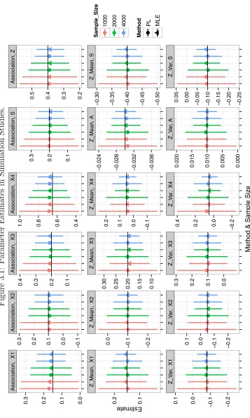
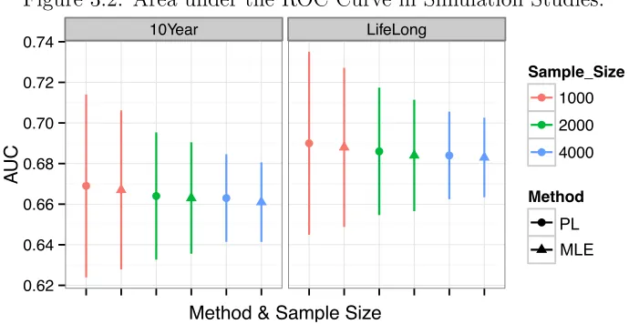
FIGURE 3.1 : Parameter Estimates in Simulation Studies. . . 50 FIGURE 3.2 : Area under the ROC Curve in Simulation Studies. . . 51

FIGURE 5.1 : Power Plot. . . 83

(13)

CHAPTER 1

(14)

1.1.

Cancer absolute risk is the probability that an individual will develop cancer in a

certain age interval without dying from competing causes. Its computation involves

the relative hazard function, the age specific baseline hazard, and age specific

com-peting risk hazard. The relative hazard function can be approximated by the odds

ratio (OR) function of the predictors since cancer outcomes are rare. The baseline

hazard rates can be calculated from composite hazard rates available from population

databases such as the Surveillance, Epidemiology, and End Results (SEER) program

when coupled with the OR function and distribution of risk predictors. The hazard

rates of mortality can be obtained from the National Death Index. This composite

approach to cancer absolute risk projection was first used by Gail et al. (1989) to

develop the breast cancer risk assessment tool (BCRAT), commonly referred to as

the ”Gail model”. The BCRAT is the current National Cancer Institute (NCI)

stan-dard for predicting breast cancer absolute risk. It has been widely used for designing

clinical trials and counseling individual woman. It can also be usefulness for selecting

high-risk women to engage in breast cancer screening programs (Saslow et al., 2007).

The BCRAT includes four risk predictors, age at menarche (Agemen), age at first

live birth (Ageflb), number of previous breast biopsies (Bbiops), and number of

first-degree relatives (Numrel) (mother/sisters) who have had breast cancer (Gail et al.,

1989). It calibrates well but only has a modest discriminatory accuracy with area

under the ROC curve (AUC) ranging from 0.58 to 0.64 (Costantino et al., 1999;

Freedman et al., 2005; Rockhill et al., 2001). Therefore, it has been of great

in-terest to increase the predictive accuracy of the BCRAT by incorporating emerging

(15)

density as the percent of dense area on the mammogram image, has recently been

established as one of the strongest risk predictors for breast cancer (Byrne et al.,

1995; Tice et al., 2008). Chen et al. (2006) and Chen et al. (2008) developed an

OR function and corresponding absolute risk prediction model that includes PD as

a new predictor, and found that it led to a modest increase in the AUC statistic.

Breast cancer risk associated SNPs, independently or in combination with PD, have

recently been extensively evaluated for their added values in improving breast cancer

risk prediction. A Swedish study showed that adding PD, body mass index, and

18 breast cancer risk SNPs can improve the AUC of a Swedish-Gail risk prediction

model from 0.55 to 0.62 (Darabi et al., 2012a). A theoretical study conducted in

the United Kingdom population showed that a 76-locus polygenetic risk score can

lead to improved risk stratification and added value more than a clinical measure of

breast density, the BI-RADS (Garcia-Closas, Gunsoy, and Chatterjee, 2014). In the

Breast Cancer Surveillance Consortium (BCSC) risk prediction model, the 76-locus

polygenetic risk score was shown to predict independently of BI-RADS breast density

(Vachon et al., 2015). It improved the BCSC model that includes BI-RADS breast

density as a predictor, increasing AUC from 0.66 to 0.69 and improving classification

of the high-risk women. To date, the combined value of PD and the 76 breast cancer

risk SNPs for improving the accuracy of the BCRAT has not been evaluated.

Notably, the evaluation of the BCRAT and other models has largely been based on

the AUC statistic, which has been argued to be of limited relevance for clinical

ap-plications. Alternative measures of predictive accuracy have been proposed, such as

predictive curves (Gail and Pfeiffer, 2005; Gu and Pepe, 2009; Pepe, Gu, and Morris,

2010; Pepe et al., 2008), the proportion of cases followed (PCF) and the proportion

(16)

de-signed for binary outcomes and are not directly applicable for evaluating absolute risk

models that were developed using the composite approach described above. In

Chap-ter 2, we adapt several existing predictive accuracy statistics to accommodate the

composite approach to absolute risk prediction, and fully evaluate the added value of

PD and/or breast cancer risk SNPs using the adapted measures, including AUC,

posi-tive predicposi-tive values(PPV), and PCF/PNF. For the BCRAT risk predictors and PD,

we use data from the Breast Cancer Detection and Demonstration Project (BCDDP).

BCDDP started in 1973 and was originally designed to assess whether mammographic

screening can reduce morbidity and mortality of breast cancer. It recruited 243,221

white women from 1973 to 1975 and followed each woman for at least 5 years. A

age-stratified case-control study was conducted in 1979, and the BCRAT risk

predic-tors were available for all 2,808 cases and 3,119 controls. But only 1,217 cases and

1,616 controls had PD measurements available. SNP genotype data is not available

from the BCDDP. Therefore, it is necessary to utilize estimates of OR parameters

and minor allele frequencies from the literature. Our proposed method of estimating

adapted accuracy statistics can accommodate these additional complications.

1.2.

The challenge of incomplete predictor data as in the BCDDP in the development

of absolute risk prediction models is widespread. For example, it may require

up-to-date high technology to measure emerging risk factors, which may be too

expen-sive or technically infeasible to use on all subjects. One such example is estrogen

metabolomic measurements. It may also be possible that genotype data cannot be

made available for all subjects. When standard risk predictors are available from

a stratified/frequency-matched case-control study but candidate predictors are only

(17)

stratified case-control design. In phase I, the case-control status and standard risk

predictors are collected on all cases and controls. In phase II, the costly predictor is

measured on a subset selected based on case-control status and phase I variables. The

incomplete data conforms to a missing at random mechanism (Little and Rubin, 1987)

because the missingness happened by study design. The development of statistical

methods for analysis has been focused on integrated analysis of phase I and phase

II data to achieve increased precision for estimating OR parameters that quantify

association between the binary outcome and risk variables (Breslow and Cain, 1988;

Breslow and Chatterjee, 1999; Breslow and Holubkov, 1997; Chen et al., 2008; Scott

and Wild, 1997). In particular, Chen et al. (2006) and Chen et al. (2008) proposed

a pseudo-likelihood approach to analyzing the two-phase stratified case-control data.

This approach was applied to analyze the BCDDP data in Chapter 2.

We are interested in developing a more efficient approach to estimating cancer

ab-solute risk, which requires efficient estimation of both OR parameters and the joint

distribution of both the standard and candidate predictors given age. Usually the

distribution of standard risk predictors can be obtained from national population

databases, which is preferable to assure the applicability of the model to the general

population. But the candidate predictor is often not included in these databases.

Therefore, our goal of efficient estimation involves that of the OR parameters and the

conditional distribution of the new predictor given standard predictors and

match-ing variables. The latter has to be estimated separately from phase II controls if

the pseudo-likelihood approach (Chen et al., 2006) is adopted for estimating the OR

parameters. In Chapter 3, we proposed a semiparametric maximum likelihood

esti-mation approach to jointly estimating the distribution of the new predictor and the

(18)

Chen et al. (2006) studied the large sample approximation of the distribution of their

proposed pseudo-likelihood estimator (Chen et al., 2006), but they did not assess the

finite sample performance nor the accuracy of the large sample approximation of the

distribution. Through extensive simulation studies and application to the analysis of

the BCDDP data, we fully evaluate the finite sample performance of our new and the

pseudo-likelihood estimators. In particular, we evaluate the corresponding efficiency

gain for estimating model parameters as well as statistics for quantifying predictive

accuracy when these approaches are used in the development of the BCRAT that

incorporates PD.

1.3.

In Chapter 4, we apply the adapted predictive measures developed in Chapter 2

to assess the incremental values of PD and 76 breast cancer risk associated SNPs

discovered to date for improving the breast cancer risk assessment tool (BCRAT)

Gail et al. (1989) for risk stratification, and thereby assess their potential in improving

model-based breast cancer screening in the United States female population. PD is

now automatically provided by most breast imaging process software. Incorporation

of PD into the BCRAT was found to lead to a modest increase in AUC Chen et al.

(2008). A small number of genetic susceptible variants for breast cancer Gail (2008);

Wacholder et al. (2010) were found to lead to a smaller increase in AUC than the PD.

But no data is available yet for quantifying the combined values of PD and breast

cancer risk SNPs in improving risk stratification in the U.S. female population. The

U.S. Preventive Task Force recommended not to routinely screen women aged 40∼49

years, which has been heavily debated by the radiology society. Therefore, we also

calculate the percentage of women in the United States aged 40∼49 years whose

(19)

1.4.

In Chapter 5, we apply the semi-parametric maximum likelihood method developed in

Chapter 2 to address the issue of survival bias in genetic association studies. Survival

bias is difficult to detect and adjust for in case-control genetic association studies

but can invalidate findings when only surviving cases are studied and survival is

associated with the genetic variants under study. We propose a design where one

genotypes genetically-informative family members (such as offspring, parents, and

spouses) of deceased cases and incorporates that surrogate genetic information into

a retrospective maximum likelihood analysis. We show that inclusion of genotype

data from first-degree relatives permits unbiased estimation of genotype association

parameters. We derive closed-form maximum likelihood estimates for association

parameters under the widely used log-additive and dominant association models.

Our proposed design not only permits a valid analysis but also enhances statistical

power by augmenting the sample with indirectly studied individuals. Gene variants

associated with poor prognosis can also be identified under this design. We provide

(20)

CHAPTER 2 Quantifying Predictive Accuracy of Cancer Absolute

(21)

2.1. Introduction

certain age period without dying from competing causes. Its computation involves

approach to cancer risk projection was used by Gail et al., 1989 to develop the breast

cancer risk assessment tool (BCRAT), commonly referred to as the ”Gail model”.

The BCRAT is the current National Cancer Institute (NCI) standard for predicting

breast cancer absolute risk. It has been widely used for designing clinical trials and

counselling individual woman. It has recently also been evaluated for its usefulness

in designing model-based breast cancer screening program.

The BCRAT uses four risk predictors, age at menarche (Agemen), age at first live

birth (Ageflb), number of previous breast biopsies (Nbiops), and number of

first-degree relatives (Numrel) (mother/sisters) who have had breast cancer. It calibrates

well but only has a modest discriminatory accuracy with area under the ROC curve

(AUC) ranging from 0.58 to 0.64 (Costantino et al., 1999; Freedman et al., 2005;

Rockhill et al., 2001). Therefore, it has been of great interest to increase the

pre-dictive accuracy of the BCRAT by incorporating emerging risk predictors. Percent

(22)

dense area on the mammogram image, has been established to be one of the strongest

risk predictors for breast cancer. Chen et al., 2006 and Chen et al., 2008 developed

an OR function and corresponding absolute risk prediction model that includes PD

as a new predictor, and found that it led to a modest increase in the AUC

statis-tic. Breast cancer risk associated SNPs, independently or combined with PD, have

recently been extensively evaluated for their added values in improving breast cancer

risk prediction. A Swedish study showed that adding PD, body mass index, and 18

breast cancer risk SNPs can improve the AUC of a Swedish-Gail risk prediction model

from 0.55 to 0.62. A theoretical study conducted in the United Kingdom population

showed that a 76-locus polygenetic risk score can lead to improved risk stratification

and added more than a clinical measure of breast density, the BI-RADS. In the Breast

Cancer Surveillance Consortium (BCSC) risk prediction model, the 76-locus

polyge-netic risk score was shown to predict independently of BI-RADS breast density. It

improved the BCSC model that also includes BI-RADS breast density as a predictor,

increasing AUC from 0.66 to 0.69 and classification of the high-risk women. But to

date, the combined value of PD and the 76 breast cancer risk SNPs for improving the

accuracy of the BCRAT has not been evaluated.

Notably, the evaluation of the BCRAT and other models has largely been based

on the AUC statistic, which has been argued to be of little relevance for clinical

applications. Alternative measures of predictive accuracy have been proposed, such as

several variants of predictive curves (Gail and Pfeiffer, 2005; Gu and Pepe, 2009; Pepe,

Gu, and Morris, 2010; Pepe et al., 2008), the proportion of cases followed (PCF) and

the proportion needed to follow up (PNF) (Pfeiffer and Gail, 2011). These measures

were designed for binary outcomes and have been adapted to time-to-event outcomes,

(23)

developed using the composite approach described above. In this chapter, we adapt

several existing predictive accuracy statistics to accommodate the composite approach

to absolute risk prediction, and evaluate the added value of PD and/or breast cancer

SNPs using the adapted measures, including AUC, positive predictive values(PPV),

and PCF/PNF. For the BCRAT risk predictors and PD, we used data from the

Breast Cancer Detection and Demonstration Project (BCDDP). BCDDP started in

1973 and was originally designed to assess whether mammographic screening can

reduce morbidity and mortality of breast cancer. It recruited 243,221 white women

in 1973 to 1975 and followed each womant for at least 5 years. An age-stratified

case-control study was conducted in 1979, and the BCRAT risk predictors were available

for all 2808 cases and 3119 controls. But only 1217 cases and 1616 controls had PD

measurements available.

We view the BCDDP data as collected from a two-phase

age-stratified/frequency-matched case-control design as in Chen et al., 2006. In phase I, the case-control

status and standard BCRAT risk predictors were collected on all cases and controls.

In phase II, PD was measured on a subset selected based on case-control status and

phase I variables. The incomplete data conforms to a missing at random mechanism

(Chen et al., 2008; Little and Rubin, 1987). To address this problem, Chen et al.

(2008) developed a pseudo-likelihood approach to deriving an OR function for breast

cancer from the BCDDP age-stratified case-control data that incorporated PD, which

we use in the absolute risk calculation in this chapter. Our estimators of adaptive

predictive accuracy statistics naturally accommodate the incomplete predictor data.

In addition, SNP genotype data is not available in the BCDDP. Therefore, it was

necessary to utilize estimates of OR parameters and minor allele frequencies from

(24)

assumed that the effects of SNPs and other non-genetic risk predictors were additive

on the logistic scale, that the OR parameters for SNPs were the same as those available

from the literature, and that the OR parameters for non-genetic risk predictors were

the same as those estimated from the BCDDP. Our proposed method of estimating

adapted accuracy statistics can accommodate these additional complications.

2.2. Methods

2.2.1. Adapted statistics for quantifying predictive accuracy of absolute risk prediction

models

Let Q denote the collection of predictors in the relative hazard function, β denote

hazard ratio parameters,λ−β denote the other Euclidean parameters that are involved

in the absolute risk prediction, and λdenote the collection of all parameters, λ=(β,

λ−β). Further, let h1(t;λ) and h2(t) denote baseline hazard rates of cancer and

competing risk hazard at age t, respectively. Then the absolute risk Ψ(Q, t0, τ;λ) in

the age interval (t0, t0+τ) can be calculated using the standard formula for cumulative

incidence function:

Ψ(Q, t0, τ;λ) =

Z t0+τ

t0

h1(u;λ)r(Q;β) exp

−

Z u

t0

{h1(v;λ)r(Q;β) +h2(v)}dv

du,

wherer(Q;β) is equal toeQβ_{and can be approximated by the OR function}_eQβ_/_{1 +}_eQβ

for rare cancer outcomes. Ideally, a cohort can be assembled from the target

popu-lation where the risk prediction model is intended to be applied to, from which all

parameters involved in Ψ(Q, t0, τ;λ) can be estimated. But this is rarely the case.

In fact, the first version of the BCRAT Gail et al. (1989) was developed based on

(25)

baseline hazard rates of breast cancer in BCDDP was higher than those in the

gen-eral U.S. female population. Therefore, for developing cancer absolute risk prediction

models, it has been popular to derive baseline hazard rates h1(t;λ) from

compos-ite hazard rates reported in population databases such as SEER. Let h∗₁(t) denote

age-specific composite hazard rates andpλ−β(Q|t) the probability distribution of pre-dictors Q at age t indexed by parameters λ−β. Then h1(t;λ) can be calculated as

h1(t;λ) = h∗₁(t){1−AR(t;λ)}, where AR(t;λ) is the attributable risk for r(Q;β) and calculated as

AR(t;λ) = 1−1/X

Q

pλ−β(Q|t)r(Q;β).

The competing risk hazard rates h2(t) can be obtained from population databases

such as the National Death Index. Define risk score Ut0(Q;β) = log{r(Q;β)} with

Q values measured at age t0. Ψ(Q, t0, τ,λ) is an increasing function of Ut0(Q;β) for

a given t0 and τ. Hereafter we write Ψ(Q, t0, τ;λ) as Ψt0,τ(Ut0;λ). The cumulative

distribution function of Ut0, denoted as F(Ut0;λ), can be estimated as ˆF(Ut0; ˆλ) =

P QI

h

Qβˆ ≤Ut0

i

ˆ p

d

λ−β(Q|t0), which is needed in the estimation of all the proposed statistics below. Let f(Ut0;λ) denote the probability density function of Ut0 and its

estimate as ˆf(Ut0;λ).

To assess the added values of breast cancer risk SNPs for improving breast cancer risk

prediction, SNP genotype data may be unavailable in studies that provide data for

non-genetic risk predictors. A compromise approach has been widely adopted that

uses OR estimates and minor allele frequencies from the literature (Gail and Pfeiffer,

2005; Gail et al., 1989). Under the assumptions that genetic and non-genetic risk

predictors are independently distributed and that their effects on breast cancer risk are

additive on the logistic scale, SNP genotypes have been incorporated into the absolute

(26)

as shown in Section 2.3 below supported this practice: estimates of the predictive

accuracy statistics are usually reasonable approximations to those when joint analysis

of SNP genotype and non-genetic risk predictor data is plausible although are a little

conservative. Therefore, this compromise approach can be useful to assess added

values for other emerging risk predictors. Suppose that there arelexternal predictors

of interest. LetW = (W1, W2, ..., Wl) denote the vector of the external predictors and

βw the corresponding log OR vector. Now the OR vector becomes (β,βw) and Q is

expanded to include W as well. Then the absolute risk is calculated using the same

formula as above, but in the calculation of attributable risk AR(t;λ),

X

Q,W

r(Q, W;β)pλ−β(Q, W |u) =

( X

Q

eQβp(Q|u)

)



 l Y

j=1



 X

Wj

eWjβwj_p₍_W j)



 





.

Adapted AUC and PPV statistic Let ψ be a pre-specified cutoff value for the

absolute risk Ψt0,τ(Ut0;λ), and T denote age at cancer diagnosis. We extend the

true positive rate (TPR) to the setting of absolute risk as the probability that an

individual who develops cancer in the age interval (t0, t0+τ), i.e. t0 < T ≤t0+τ, is classified as high risk at t0 by the criteria Ψt0,τ ≥ψ,

TPRψ(t0, τ;λ) = p[Ψt0,τ(Ut0;λ)≥ψ|t0 < T ≤t0+τ].

Similarly, We define the false positive rate (FPR) as the probability that an individual

who remains cancer-free by aget0+τ, i.e. T > t0+τ, is classified as high risk,

FPRψ(t0, τ;λ) = p[Ψt0,τ(Ut0;λ)≥ψ|T > t0+τ].

(27)

TPR_FPR−1₍_t

0,τ;λ)(t0, τ;λ).

We propose a model-based approach to the estimation of the adapted AUC statistic.

To estimate TPR, we re-write it using the Bayes rule

TPRψ(t0, τ;λ) =

p[Ψt0,τ(Ut0;λ)≥ψ, t0 < T ≤t0+τ] p(t0 < T ≤t0+τ)

=

P

Ut₀I[Ψt0,τ(Ut0;λ)≥ψ]p[Ut0, t0 < T ≤t0+τ] P

Ut0 p[Ut0, t0 < T ≤t0+τ] =

P

Ut₀I[Ψt0,τ(Ut0;λ)≥ψ]p[t0 < T ≤t0+τ|Ut0]p(Ut0)

P

Ut₀ p[t0 < T ≤t0+τ|U]p(Ut0) =

P

Ut₀I[Ψt0,τ(Ut0;λ)≥ψ] Ψt0,τ(Ut0;λ)f(Ut0;λ)

P

Ut0 Ψt0,τ(Ut0;λ)f(Ut0;λ)

.

Then TPR can be estimated as

[

TPRψ(t0, τ;λ) =

P Ut0 I

h

Ψt0,τ(Ut0; ˆλ)≥ψ

i

Ψt0,τ(Ut0; ˆλ) ˆf(Ut0; ˆλ)

P

Ut0 Ψt0,τ(Ut0; ˆλ) ˆf(Ut0; ˆλ)

.

Similarly, FPR can be estimated as

[

FPRψ(t0, τ;λ) =

P Ut₀ I

h

i h

1−Ψt0,τ(Ut0; ˆλ)

i

ˆ

f(Ut0; ˆλ)

P Ut₀

h

1−Ψt0,τ(Ut0; ˆλ)

i

ˆ

f(Ut0; ˆλ)

.

Then the AUC statistic can be estimated as TPR[ [

FPR−1(t0,τ; ˆλ)(t0, τ; ˆλ).

Similar as TPR, we define PPV as the probability that an individual whose absolute

risk at age t0 is above threshold ψ, Ψt0,τ ≥ψ, will develop cancer in the age interval (t0, t0 +τ):

(28)

Similar as the estimation of TPR/FPR above, we propose a model-based estimator

as

[

PPVψ(t0, τ; ˆλ) =

P Ut₀ I

h

i

Ψt0,τ(Ut0; ˆλ) ˆf(Ut0; ˆλ)

P Ut0 I

h

i

ˆ

f(Ut0; ˆλ)

.

Adapt the PCF/PNF statistics to the absolute risk projection PCF at percentage

q, written as PCF(q), is defined as the proportion of individuals who develop cancer

in age interval (t0, t0 +τ) among those whose absolute risk exceeds the (1−q)th percentile in the target population. PNF at percentagepis defined as the proportion

of the population at highest risk that is needed to be followed so that a proportionp

of those destined to develop cancer in the age interval (t0, t0+τ) will be captured. Let

G(ψ;λ) denote the cumulative distribution function of the absolute risk Ψt0,τ(Ut0;λ),

G(ψ;λ) =p[Ψt0,τ(Ut0;λ)≤ψ] =

X

Ut₀

I[Ψt0,τ(Ut0;λ)≤ψ]f(Ut0;λ).

We estimate PCF(q) as PCF([ q; ˆλ):

[

PCF(q; ˆλ) =

P Ut₀ I

h

Ψt0,τ(Ut0; ˆλ)≥G

−1₍₁₋_q₎i_Ψ

t0,τ(Ut0; ˆλ) ˆf(Ut0; ˆλ)

P

Ut₀ Ψt0,τ(Ut0; ˆλ) ˆf(Ut0; ˆλ)

By definition, PNF is the inverse function of PCF. That is,

pΨt0,τ(Ut0;λ)≥G −1

[1−PNF(p)]|t0 ≤T ≤t0+τ =p.

Therefore, PNF can be estimated by inverting the PCF estimate PCF([ q; ˆλ).

Large sample distribution of the adpated statistics Let P AS(λ) denote any of

(29)

statistics”. The estimators that we proposed above can all be written as P AS( ˆλ)

, where ˆλ is consistent estimators of λ. Assume that ˆλ is asymptotically normally

distributed with meanλ and variance Σλ. Based on Taylor series expansion, we can

show that P AS[ ∼N(P AS,Σ).

Here the variance of P AS is estimated by ˆΣ, which is derived using Talor series

expansion. Thus

ˆ Σ =

"

∂P AS( ˆλ) ∂λ

#

ˆ Σλ

"

∂P AS( ˆλ) ∂λ

#

,

where ˆΣλis consistent estimator for Σλ. We provide the theoretical asymptotic results

in the Appendix.

We present as follows the forms for ∂T P R_∂_λ( ˆλ)as examples for ∂P AS_∂_λ( ˆλ). The other

ex-pressions of the first derivatives over λ and fU can be derived similarly.

∂T P R[ψ(t0, τ; ˆλ)

∂λ =

P U

h ∂Iˆ

∂λΨ ˆˆf + ˆI ∂Ψˆ

∂λfˆ+ ˆIΨˆ ∂fˆ ∂λ i

P UΨ ˆˆf

−

h P

UIˆΨ ˆˆf i n

P U

h ∂Ψˆ

∂λfˆ+ ˆΨ ∂fˆ ∂λ

io

h P

UΨ ˆˆf i2

where ˆI, ˆΨ and ˆf are the estimated indicator function, absolute risk function and joint

distribution of the predictors involved in the formulas of TPR. Number of predictors

in the cancer absolute risk prediction model can be very large since the distribution

of predictors given age can be estimated empirically. The dimension of Varλˆ will

be very high (probably as large as several hundreds), which makes the estimation of

the variance difficult. Therefore in practice, we calculate the variance of each statistic

(30)

2.2.2. Estimation of parameters λ with two-phase stratified case-control data

Motivated by the BCDDP, we consider that the relative risk/OR parameters β are

estimated from two-phase stratified case-control data, where one or more predictors

in Q are observed only in a selected subset of cases and controls. Chen et al. (2006)

proposed a general pseudo-likelihood (PL) approach to estimation, which we adopt

in the estimation of absolute risk and statistics P AS{λ, f(Ut0;λ)}. The PL method stratified on standard risk factors and the matching variable. However, the data would

be too sparse after stratification. Methods for analyzing two-phase case-control data

(Breslow and Chatterjee, 1999; Breslow and Holubkov, 1997) are applicable to the

analysis of two-phase stratified case-control data. These methods utilize data on fully

observed predictors and thereby improve the efficiency of estimating OR parameters

through post stratification. But the consistency of these methods require stratification

on the sampling variables when applied to two-phase stratified case-control data.

This leaves little room for post-stratifying on the fully observed predictors, because

reasonable stratum sizes (rule of thumb is greater than 5) are necessary to ensure

finite sample performance. Recognizing that OR parameters for sampling variables

are not of interest, PL ignored phase I sampling variables and post-stratified only on

fully observed risk predictors.

LetY denote the case-control status, A denote the matching variable, andX denote

risk predictors. Data on X is collected for n1 cases andn0 controls who are matched

on A, which is discrete and takes a small number of values. Let Z denote a single

predictor that is collected only on a subset of m1 cases and m0 controls (m1 ≤ n1, m0 ≤ n0). Often, auxiliary information for Z is available in phase I which can be exploited to increase efficiency for estimating the OR parameter for Z. For example,

(31)

PD. These auxiliary variables can be included in predictors X. The case-control

status Y is related toQ= (X, Z) via a logistic regression model

logitp(Y = 1||Q, A) =αa+βTQ, (2.1)

where αa is the sampling-stratum specific intercept parameter. The PL method for

estimating OR parameters β requires that the number of subjects with outcome

Y = y within each matching stratum A = a, Nya, in the cohort from which cases

and controls were assembled is known. Let nya denote such number in the

case-control study. Further, let K(X) denote a coarsened version of X for defining

post-stratification strata, which can be X itself when X is discrete with a small number

of levels. The PL method treated the stratified case-control sample as prospective

that conforms to the logistic regression model (2.1) but with a modified intercept to

adjust for case-control sampling

p∗(Y =y|X, Z, A) = exp

y α∗_a+β_xTX+βzZ

1 + exp{(α∗

a+βxTX+βzZ)}

,

where α∗_a = αa+ log (n1aN0a/n0aN1a). The PL takes the form of the standard

like-lihood for the two-phase design with phase I data generated prospectively from the

modified model p∗(Y =y|X, Z, A), and the logarithm of which was given as

`P L =

m1+m0

X

i=1

log{p∗(Yi|Xi, Zi, Ai)p∗[Xi, Zi, Ai|K(Xi)]}+ n1

X

i=m1+1

log{p∗(Yi|K(Xi))}

=

m1+m0

X

i=1

log{p∗(Yi|Xi, Zi, Ai)p∗(Xi, Zi, Ai|K(Xi))}

+

n1

X

i=m1+1 log

Z

p∗(Yi|Xi, Z, Ai)p∗[Xi, Z, Ai|K(Xi)]dZ

(32)

`P L is a log pseudo-likelihood but not a genuine likelihood becausep∗(Y =y|X, Z, A)

is not a real probability density function. Chen et al. (2008) showed that maximizing

`P L yields a consistent estimate of β and studied large sample properties of the

estimator ˆβ.

Estimation of absolute risk and P AS also requires estimation of parameters in the

risk predictor distribution p(Q). Under the two-phase stratified case-control design,

one can appropriately model the conditional distribution pθ(Q|A), where θ is the

associated parameter vector, and estimate model parametersθ using data from phase

II controls. When the distribution for the matching variableA can be obtained from

external resources, p(Q) can be obtained asp(Q) =P

Apθ(Q|A)p(A).

2.3. The analysis of BCDDP data

We applied the developed methods to compare the predictive accuracy of four

mod-els for breast cancer absolute risk: BCRAT, BCRAT plus breast cancer risk SNPs,

BCRAT plus PD and weight, and BCRAT plus breast cancer risk SNPs, PD, and

weight. The ORs in the third model and those for non-genetic risk predictors in the

forth model were estimated by applying the PL method to the BCDDP data.

Previ-ous work used BMI rather than weight when modeling PD on breast cancer risk to

recognize the strong confounding effect of BMI. But only weight was available from

the BCDDP. We used 74 SNPs instead of 76 as in previous work because two of the

SNPs were not statistically significant in a recent meta analysis. The PL method

efficiently used data on variables Agemen, Nbiops, Ageflb, Numrel, and Weight that

(33)

2.3.1. Absolute risk estimation and predictive accuracy statistics with the BCDDP

data and external SNP predictors

We describe the detailed methods for developing and evaluating the three variant

BCRAT models above. Denote the four standard predictors and weight as X =

(X1, X2, X3, X4, X5), PD asZ, so that Q= (X, Z), and the external 74 breast cancer

risk SNPs as W = (W1, W2, ..., W74). The controls were frequency-matched to cases

on age,A, in 5-year intervals, so that the sampling variableAhere agrees witht0in the

absolute risk formula in section 2.2.1. Therefore, the predictor distribution given age

u in section 2.2.1, pλ−β(Q|u), and the predictor distribution given matching variable A in section 2.2.2, pθ(Q|A) concide. Below we express this distribution by pθ(Q|A).

We used the same numerical coding for (X1, X2, X3, X4, A) as in the BCRAT and

in Chen et al. (2008), and each component of W were coded as 0, 1, or 2 for the

minor allele count. We codedZ slightly different, however. Previous work categorized

PD into quartiles where the first quartile [0,0.25) includes value 0. However, Z = 0

may indicate a genuine zero dense area but more likely suggests that a woman’s

dense area on the mammographic image was below the detection limit. Therefore,

we treated Z = 0 as a separate category resulting in 5 categories of PD. Denote the

corresponding categorized Z as Zc_{. The joint distribution of the predictors given}

A, p(Q, W|A), which can be factorized as pθ(Zc|X, A)p(X|A)p(W). Similar as the

BCRAT, we estimatedp(X|A) non-parametrically from the National Health Interview Survey (NHIS). We approximated pθ(Zc|X, A) by the same distribution in controls,

pθ(Zc|X, A;Y = 0). We model the continuous PD measure Z by a zero-inflated beta

regression modelpθ(Z|X, A;Y = 0), so thatpθ(Zc|X, A) = R

Ωcpθ(Z|X, A;Y = 0)dZ,

where Ωc is the support for Zc. In addition, the 74 breast cancer risk SNPs were

(34)

Equilibrium law, so that p(W) =Q74

j=1p(Wj), p(Wj = 0) = (1−pwj)

2_, _p₍_W

j = 1) =

2pwj(1−pwj), p(Wj = 2) =p

2

wj, E [Wj] = 2pwj, and Var [Wj] = 2pwj 1−pwj

.

The calculation of absolute risk involves the OR parameter estimates and the

distri-bution of the risk predictors. Instead of doing integration as shown in the absolute

risk formula, we sum over the age interval (A, A+τ) by treating the age variable A

as discrete numbers (e.g., 21,22,23, ...). However, A remains to be continuous in the

computation ofpθ(Zc|X, A;Y = 0).

The estimation of the distribution of UA = Qβ +W βw, f(UA;λ), which is needed

in the calculation of all the predictive accuracy statistics, requires enumeration of all

possible combined values of (Q, W) = (X, Zc_{, W}_{). But this is infeasible because of}

the large number of SNPs. Therefore, instead of obtaining the exact distribution of

(Q, W) at ageA, we used the large sample approximation by resorting to the Central

Limit Theorem, so that UA is asymptotically normally distributed with mean and

variance

E[UA] = E [Xβx+Zcβz |A] + E [Wβw |A]

= X

X,Zc

(Xβ_x+Zcβz) Z

Ωc

pθ(Z |X, A;Y = 0)dZ

p(X |A) + 74

X

j=1

(35)

and

Var[UA] = Var [Xβx+Zcβz |A] + Var [Wβw |A]

= E

(Xβ_x+Zcβz)2 |A

−E2[Xβ_x+Zcβz |A] +

74

X

j=1 Var

βwjWj

= X

X,Zc

(Xβ_x+Zcβz)2 Z

Ωc

p(X|A)

−

( X

X,Zc

(Xβ_x+Zcβz) Z

Ωc

p(X |A)

)2

+ 74

X

j=1

β_w2_jVar [Wj].

With the resultant asymptotic distribution f(UA;λ), we calculated AUC, PPV, and

PCF based on the formulas in previous sections.

2.3.2. Results

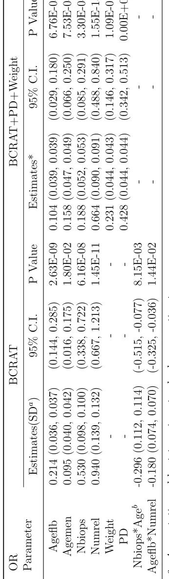
The OR parameter estimates for variables in the BCRAT and BCRAT+PD+Weight

models are provided in Table 2.1. Note that the two interaction terms that were

included in the BCRAT were not significant in the BCRAT+PD+Weight model and

therefore excluded. The OR estimates for the two strongest risk predictors, Nbiops

and Numrel, became much smaller in the latter model, which may be due to the

correlation between PD and Nbiops and Numrel as shown in Chapter 3. Our

es-timates were slightly different from those in Chen et al. (2008), because we used

coarser post-stratification strata in the PL method. This is mainly to facilitate the

bootstrapping method for obtaining asymptotic variance estimates of the predictive

accuracy statistics. The coarser strata guaranteed that the same post-stratification

can guarantee a reasonable size of each stratum in each bootstrapping sample. The

(36)

T able 2.1: Estimates of the OR P arameters for BCDDP .

OR Parameter

(37)

circumstances.

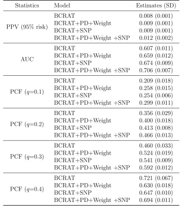
Table 2.2: Estimates of Predictive Accuracy Statistics for the BCRAT and its Vari-ants.

Statistics Model Estimates (SD)

PPV (95% risk)

BCRAT 0.008 (0.001) BCRAT+PD+Weight 0.009 (0.001) BCRAT+SNP 0.009 (0.001) BCRAT+PD+Weight +SNP 0.012 (0.002)

AUC

PCF (q=0.1)

PCF (q=0.2)

PCF (q=0.3)

PCF (q=0.4)

The estimates of predictive accuracy statistics for the four models are provided in

Table 2.2. The standard deviations were obtained by bootstrapping 1000 samples

from the BCDDP. We first generated 1000 samples from the original data by sampling

with replacement from each stratum defined by case-control status and age groups.

With each bootstrapping sample, we estimated (β,θ). Then we applied parametric

(38)

variance-covariance matrix from NHIS dataset. Finally, we parametrically bootstrapped 1000

sets ofβ_wwith the estimated log ORs and variances from literature. We then obtained

1000 sets of estimates ( ˆβ,θˆ) and ˆp(X|A). The standard errors of each statistic is then calculated from the 1000 corresponding predictive accuracy statistics. The calculation

of all predictive accuracy statistics was based on the 5-year risk for 35 year old women.

Adding SNPs and PD lead to large improvement in all predictive accuracy statistics,

and SNPs appeared to have a slightly larger incremental value. PPV was 0.54%,

0.71%, 0.70%, and 0.82% under the BCRAT, BCRAT+PD+Weight, BCRAT+SNP,

and BCRAT+PD+Weight+SNP, respectively. The PPV of the BCRAT was 0.0075,

suggesting that 0.75% of the 35 year-old women whose breast cancer absolute risk

was greater than 0.54% (top 5%, high risk) will develop breast cancer by age 40.

The PPV for the other three models were 0.93%, 0.93%, and 1.17%, respectively.

The AUC statistic under the four models were 0.607, 0.659, 0.674, and 0.706. We

computed PCF under different q values. At q = 0.2, the PCF for the four models

were 0.356, 0.400, 0.413, and 0.466, respectively. These results indicated that for the

35 year-old women who will develop breast cancer in the age interval (35, 40), 11%

more will arise among women whose absolute risk exceeds the 80% percentile in the

population as calculated by each model. PCF at the other q values showed similar

results.

2.4. Simulation Study

We then conducted extensive simulation studies to 1) assess the finite sample

perfor-mance of the asymptotic standard error estimates for predictive accuracy statistics,

and 2) assess the performance of normal approximation to the distribution of risk

(39)

in-corporated from external sources. We designed the simulation studies so that the

distribution of risk predictors was similar to that in the BCDDP. Therefore, we

ex-pect that our simulation results will also yield insights on the performance of variant

BCRAT models.

To generate two-phase stratified case-control samples, we first simulate a population

under the true model with all predictors and SNPs as follows. We first generated for

each subject data on age A, five predictors X = (X1, X2, X3, X4, Z), and external

predictors W = (W1, W2, ..., Wl). The age group indicatorIA was obtained as IA = 1

for 30 ≤ A < 40, IA = 2 for 40 ≤ A < 50, IA = 3 for 50 ≤ A < 60, IA = 4 for

60≤A <70, andIA= 5 forA≥70, whereAwas generated from a uniform

distribu-tion Uniform(30,80). X1 took values 0, 1, 2 and 3 and X2 values 0, 1 and 2 with the

frequency of each value similar to that of Ageflb and Agemen in the BCDDP,

respec-tively. X3 were generated from Poisson(0.8) and X4 from Poisson(0.2) by assigning

values 0, 1, and 2 to categories 0, 1, and ≥2, respectively. We generated the contin-uous Z measurement from Beta distribution, Beta(κφ, φ−κφ), with logit(κ) = Qγ

and log(φ) = Qω, where Q = (1, X, A), and we used for parameters θ = (γ,ω)

similar values as the corresponding estimates in the BCDDP. Then we categorized

Z to create variable Zc _{taking values 0, 1, 2 and 3 for} _Z _∈ ₍₀_,₀_._{25), [0}_.₂₅_,₀_._50),

[0.50,0.75) and [0.75,1), respectively. We generated l independent SNPs, with the

genotype data for each SNPj generated from a multinomial distribution with values

0, 1 and 2 and corresponding probabilities (1−pj)2, 2pj(1−pj) and p2j, wherepj was

the minor allele frequency for the jth SNP and j = 1,2, ..., l. Finally, we generated

case-control status Y from a Bernoulli distribution with probability

(40)

We treated all predictors as ordinal in the analyses. We then randomly sampled n/5

cases andn/5 controls from each age stratum using variable probability sampling, so

that each case-control sample includedn cases andn controls. To create a two-phase

design sample, we randomly sampled a subset of cases and controls stratifying on A

and then deleted data Zc _{for the rest of case-control subjects.}

The estimation of the predictor distribution p(X, Zc, W|A), as required in the esti-mation of predictive accuracy statistics, requires estimates of parameters θ in the

distributionpθ(Zc|X, A),p(X|A), andpj. For each dataset, we estimatedθ by fitting

a beta regression model to phase II controls only. Because p(X|A) and pj were

gen-erally estimated from external resources, we keep them fixed in the simulation. To

evaluate the normal approximation to the distribution of risk scoreXβ_x+Zc_β

z+Wβw

when the number of SNPs is large, we compared results obtained with normal

approx-imation and those with the exact distribution. For the former, we estimated (β_x, βz)

for each simulated dataset by fitting model (2.2) but withoutW using the PL method,

and estimatedβ_w from an independent case-control sample generated from the same

population as described by model (2.2). For the latter, we jointly estimated (β_x, βz)

andβ_w by fitting model (2.2) using the PL method, and we refer to the corresponding

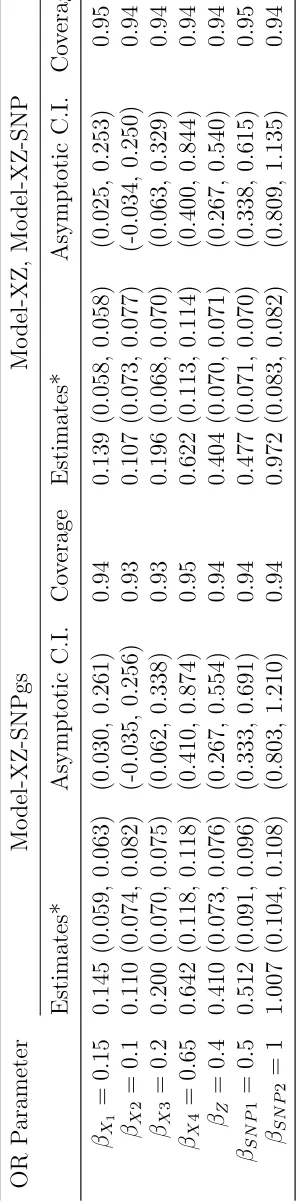
estimates of predictive accuracy statistics as “gold standard”. We considered 2 SNP

predictors in W to make the computation of the exact distribution feasible in this

comparison. Below, We used “Model-XZ” to refer a the model that only used (X, Z)

as predictors, “Model-XZ-SNP” a model that includes both (X, Z) and W but with

(β_X, βz) and βw estimated separately as above, and “Model-XZ-SNPgs” the “gold

standard” model.

As shown in Table 2.3, even if we used intentionally large OR values for the two

(41)

(42)

regardless of whether they were estimated jointly or separately, and the asymptotic

standard error estimates were close to the empirical estimates as well. The 95%

confidence intervals provided good coverages as well. Therefore, the potential bias

resulting from fitting a mis-specified model (“Model-XZ”) due to omission of the

two SNPs is small. This observation is owing to the fact that the outcome Y was

rare and that SNPs and the rest of the predictors were independently distributed in

the population. Because we considered strong SNP effects, this same observation is

expected to be generalizable to when a larger number of SNPs with weaker SNPs are

related, as in the variant BCRAT models.

The estimates of predictive accuracy statistics and their standard errors are presented

in Table 2.4. PPV was computed at the 95% absolute risk quantile cutoff, which,

un-der Model-XZ-SNP, was quite close to that unun-der Model-XZ-SNPgs. PPV estimates

were the largest under Model-XZ-SNPgs as expected, and those under

model-XZ-SNP was similar. The average asymptotic and empirical standard errors were close.

For the two SNPs, except for the OR values in Table 2.3, β_w = (0.5,1), we also

considered weaker effects β_w = (0.3,−0.15) and stronger effects β_w = (1,2). The results were largely the same (data not shown). The AUC statistic under the three

models were 0.679, 0.744, and 0.752, respectively. We calculated PCF at different q

values, 0.1, 0.2, 0.3 and 0.4 . Model-XZ-SNP and Model-XZ-SNPgs always had

sim-ilar PCFs, which were greater than that under Model-XZ. As shown by PPV, AUC,

and PCF statistics, although Model-XZ-SNP is a composite approach to evaluating

the predictive accuracy, it performed similar as the gold standard one. In

particu-lar, Model-XZ-SNP led to a conservative assessment of the added value of Z, and

therefore is an appealing first step to assess a potential risk predictor. The average

(43)

latter was slightly smaller.

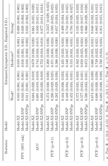
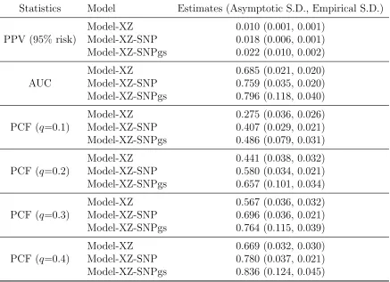
Finally, we performed simulation studies withW including 74 SNPs as in the variant

(44)

BCDDP model (Table 2.5). Due to the large number of SNPs, we adopted normal

approximation to the risk score Xβ_x +Zc_β

z +Wβw when computing predictive

accuracy statistics under both “Model-XZ-SNP” and “Model-XZ-SNPgs”. We used

the exact distribution for Xβ_x+Zc_β

z under “Model-XZ”. As observed for the

two-SNP setting, for all the predictive accuracy statistics, we observed large improvement

of Model-XZ-SNP over Model-XZ, and those under Model-XZ-SNPgs were usually

noticeably larger that those under Model-XZ-SNP. For all statistics, the asymptotic

standard error estimate was usually larger than empirical standard error, although

they were reasonably close for Model-XZ and Model-XZ-SNP. The large discrepancy

under Model-XZ-SNPgs might be due to the large dimension of variance-covariance

matrix for the large number of OR parameters. Statistics under Model-XZ-SNP, most

of the time, had smaller empirical standard errors than those under Model-XZ.This

was because Model-XZ-SNP exploited external information for SNP OR parameters

and minor allele frequencies, which were treated as known. Our results suggested

that normal approximation could lead to reasonable albeit conservative assessment

(45)

Table 2.5: Estimates of Predictive Accuracy Statistics in Simulation Studies with 74 SNPs.

Statistics Model Estimates (Asymptotic S.D., Empirical S.D.)

PPV (95% risk)

Model-XZ 0.010 (0.001, 0.001) Model-XZ-SNP 0.018 (0.006, 0.001) Model-XZ-SNPgs 0.022 (0.010, 0.002)

AUC

PCF (q=0.1)

PCF (q=0.2)

PCF (q=0.3)

PCF (q=0.4)

2.5. Conclusion

The estimators that we proposed for the adapted statistics were model-based,

treat-ing the absolute risk model as the correct model to relate risk predictors and the

probability of developing breast cancer. But this is rarely true in reality. The same

issue arose for predicting binary and time-to-event outcomes, where nonparametric

estimation methods were proposed that were robust to model mis-specification.

How-ever, in the setting of the widely applied composite approach to the development of

cancer absolute risk prediction models, nonparametric estimation methods are not

(46)

and events. Our method allows investigators to have at least an initial look at the

added values of candidate predictors.

The efficiency of estimating the adapted statistics depends on the efficiency of

es-timating the OR association parameters and the distribution of risk predictors. In

our current work, the PL method is not fully efficient for estimating OR association

parameters, and parameters in the conditional distribution of the new predictor was

estimated from phase II controls. It is of great interest to develop more efficient

methods for estimation. In Chapter 3, we propose a semiparametric maximum

likeli-hood approach (MLE) to estimating these two sets of parameters, which is expected

to lead to more efficient estimates of the adapted accuracy statistics. On the other

hand, the PL method is robust to the specification of the distribution of the new

predictor, but the semiparametric MLE can yield biased estimates of OR parameters

if the distribution of the new predictor is mis-specified. This bias and efficiency trade

off needs to be carefully considered for deciding which method to use in data analysis.

Our evaluation of combined values of PD and breast cancer risk SNPs relied on

multiple assumptions in order to utilize data in the literature on SNP minor allele

frequencies and OR parameter estimates. But SNPs may contribute to the variation

in the distribution of non-genetic risk predictors such as PD and family history of

breast cancer, and estimates of the OR parameters in the literature from marginal

analysis are biased for those in the logistic model that includes both genetic and

non-genetic risk predictors. Nevertheless, in the absence of data that provides information

on all predictors, this approach allows initial exploration of the combined values of all

predictors. Our simulation studies indicated that this approach provides reasonable

approximation at least for breast cancer risk prediction in the general female

(47)

in estimating the added values. Our results showed that incorporating PD and the

74 breast cancer risk SNPs improves the predictive accuracy of the BCRAT in term

(48)

CHAPTER 3 Semiparametric Maximum Likelihood Estimation with

(49)

3.1. Introduction

certain age period without dying from competing causes. Its computation involves

approach to cancer risk projection was first used by Gail et al. (1989) to develop the

breast cancer assessment tool (BCRAT), commonly referred to as the “Gail model”.

The BCRAT is the current National Cancer Institute (NCI) standard for predicting

breast cancer absolute risk. It has been widely used for designing clinical trials and

counseling individual woman. It has recently also been evaluated for its usefulness in

designing model-based breast cancer screening program.

The BCRAT includes four risk predictors, age at menarche (Agemen), age at first

live birth (Ageflb), number of previous breast biopsies (Bbiops), and number of

first-degree relatives (mother/sisters) (Numrel) who had breast cancer. It calibrates well

but only has a modest discriminatory accuracy with the area under the ROC curve

(AUC) ranging from 0.58 to 0.64 (Costantino et al., 1999; Freedman et al., 2005;

Rockhill et al., 2001). Therefore, it has been of great interest to increase the

pre-dictive accuracy of the BCRAT by incorporating emerging risk predictors. Percent

(50)

dense area on the mammogram image, has recently been established to be one of the

strongest risk predictors for breast cancer. Chen et al. (2006) and Chen et al. (2008)

developed an OR function and the corresponding absolute risk prediction model that

included PD as a new predictor, and found that it led to a modest increase in the

AUC statistic. Breast cancer risk associated SNPs, independently or combined with

PD, have recently been extensively evaluated for their added values in improving

breast cancer risk prediction. In Chapter 2, we adapted several statistics for

evaluat-ing the accuracy of models developed with binary or time-to-event outcome data to

accommodate the composite approach to absolute risk prediction, and assessed the

combined value of PD and the 74 breast cancer risk SNPs for improving the accuracy

of the BCRAT.

In Chapter 2, for the BCRAT and its variants, we used data for risk predictors

and PD from the Breast Cancer Detection and Demonstration Project (BCDDP).

BCDDP started from 1973 and was originally designed to assess whether

mammo-graphic screening can reduce morbidity and mortality of breast cancer. It recruited

243,221 white women in 1973 to 1975 and followed up each subject for at least 5

years. An age-stratified case-control study was conducted in 1979, and the BCRAT

risk predictors were available for all 2808 cases and 3119 controls. But only 1217

cases and 1616 controls had PD measurements available. SNP genotype data was

not available from the BCDDP. The challenge of incomplete predictor data as in the

BCDDP in the development of absolute risk prediction models is widespread. For

example, it may require up-to-date high technology to measure emerging risk factors,

which may be too expensive or technically infeasible to use on all subjects. One such

example is estrogen metabolomic measurements. It may also be possible that

(51)

are available from a stratified/frequency-matched case-control study but candidate

predictors are only collected on a subset, the data can be viewed as arising from

a two-phase stratified case-control design. In phase I, the case-control status and

standard risk predictors are collected on all cases and controls. In phase II, costly

predictor is measured on a subset selected based on case-control status and phase I

variables. The incomplete data conforms to a missing at random mechanism (Little

and Rubin, 1987) because the missingness occurred by study design. The

develop-ment of statistical methods for analysis has been focused on integrated analysis of

phase I and phase II data to achieve increased precision for estimating OR parameters

that quantify associations between the binary outcome and risk variables (Breslow

and Cain, 1988; Breslow and Chatterjee, 1999; Breslow and Holubkov, 1997; Chen

et al., 2008; Scott and Wild, 1997). In particular, Chen et. al (2006, 2008) carried

out a pseudo-likelihood approach to analyzing the two-phase stratified case-control

data and derive the OR function. This approach was applied to analyze the BCDDP

data in Chapter 2.

We are interested in developing a more efficient approach to estimating cancer

ab-solute risk and predictive accuracy statistics developed in Chapter 2, which requires

efficient estimation of both OR parameters and the joint distribution of standard and

candidate predictors given age. Usually the distribution of standard risk predictors

can be obtained from national population databases, which is preferable to assure the

applicability of the model to the general population. But candidate predictors are

often not included in these databases. Therefore, our goal involves efficient estimation

of the OR parameters and conditional distribution of the candidate predictor given

standard predictors and age. Here, we propose a semiparametric maximum

Cancer Absolute Risk Projection with Incomplete Predictor Variables

University of Pennsylvania

ScholarlyCommons

Cancer Absolute Risk Projection with Incomplete

Predictor Variables

Lu Chen

Cancer Absolute Risk Projection with Incomplete Predictor Variables

ACKNOWLEDGEMENT

ABSTRACT

TABLE OF CONTENTS

LIST OF TABLES

LIST OF ILLUSTRATIONS

CHAPTER 1

1.1.

1.2.

1.3.

1.4.

CHAPTER 2

Quantifying Predictive Accuracy of Cancer Absolute

2.1. Introduction

2.2. Methods

2.3. The analysis of BCDDP data

2.4. Simulation Study

2.5. Conclusion

CHAPTER 3

Semiparametric Maximum Likelihood Estimation with

3.1. Introduction