Statistical Methods for Analysis of Multi-Sample Copy Number Variants and ChIP-seq Data

(1)

University of Pennsylvania

ScholarlyCommons

Publicly Accessible Penn Dissertations

1-1-2013

Statistical Methods for Analysis of Multi-Sample

Copy Number Variants and ChIP-seq Data

Qian Wu

University of Pennsylvania, wuqian7@gmail.com

Follow this and additional works at:http://repository.upenn.edu/edissertations Part of theBiostatistics Commons

This paper is posted at ScholarlyCommons.http://repository.upenn.edu/edissertations/948

For more information, please contactlibraryrepository@pobox.upenn.edu. Recommended Citation

Wu, Qian, "Statistical Methods for Analysis of Multi-Sample Copy Number Variants and ChIP-seq Data" (2013).Publicly Accessible

Penn Dissertations. 948.

(2)

Statistical Methods for Analysis of Multi-Sample Copy Number Variants

and ChIP-seq Data

Abstract

This dissertation addresses the statistical problems related to multiple-sample copy number variants (CNVs) analysis and analysis of differential enrichment of histone modifications (HMs) between two or more biological conditions based on the Chromatin Immunoprecipitation and sequencing (ChIP-seq) data. The first part of the dissertation develops methods for identifying the copy number variants that are associated with trait values. We develop a novel method, CNVtest, to directly identify the trait-associated CNVs without the need of identifying sample-specific CNVs. Asymptotic theory is developed to show that CNVtest controls the Type I error asymptotically and identifies the true trait-associated CNVs with a high probability. The performance of this method is demonstrated through simulations and an application to identify the CNVs that are associated with population differentiation.

The second part of the dissertation develops methods for detecting genes with differential enrichment of histone modification between two or more experimental conditions based on the ChIP-seq data. We apply several nonparametric methods to identify the genes with differential enrichment. The methods can be applied to the ChIP-seq data of histone modification even without replicates. It is based on nonparametric hypothesis testing in order to capture the spatial differences in protein-enriched profiles. The key of our approaches is to use null genes or input ChIP-seq data to choose the biologically relevant null values of the tests. We demonstrate the method using ChIP-seq data on a comparative epigenomic profiling of adipogenesis of murine adipose stromal cells. Our method detects many genes with differential H3K27ac levels at gene promoter regions between proliferating preadipocytes and mature adipocytes in murine 3T3-L1 cells. The test statistics also correlate well with the gene expression changes and are predictive of gene expression changes, indicating that the identified differential enrichment regions are indeed biologically meaningful.

We further extend these tests to time-course ChIP-seq experiments by evaluating the maximum and mean of the adjacent pair-wise statistics for detecting differentially enriched genes across several time points. We compare and evaluate different nonparametric tests for differential enrichment analysis and observe that the kernel-smoothing methods perform better in controlling the Type I errors, although the ranking of genes with differentially enriched regions are comparable using different test statistics.

Degree Type Dissertation Degree Name

Doctor of Philosophy (PhD) Graduate Group

Epidemiology & Biostatistics First Advisor

(3)

Keywords

ChIP-seq, CNV, Histone modification, Kernel-smoothing, Multi-sample, Nonparametric test Subject Categories

Biostatistics

(4)

STATISTICAL METHODS FOR ANALYSIS OF MULTI-SAMPLE COPY NUMBER VARIANTS AND CHIP-SEQ DATA

Qian Wu

A DISSERTATION

in

Epidemiology and Biostatistics

Presented to the Faculties of the University of Pennsylvania

in

Partial Fulfillment of the Requirements for the

Degree of Doctor of Philosophy

2013

Supervisor of Dissertation

Hongzhe Li, Professor of Biostatistics

Graduate Group Chairperson

Daniel F. Heitjan, Professor of Biostatistics

Dissertation Committee

Mingyao Li, Associate Professor of Biostatistics Sarah Ratcliffe, Associate Professor of Biostatistics

(5)

STATISTICAL METHODS FOR ANALYSIS OF MULTI-SAMPLE COPY

NUMBER VARIANTS AND CHIP-SEQ DATA

c

COPYRIGHT

2013

Qian Wu

This work is licensed under the Creative Commons Attribution NonCommercial-ShareAlike 3.0 License

To view a copy of this license, visit

(6)

ACKNOWLEDGEMENT

I have a lot of good memories and experiences at Penn. During the completion of my

Ph.D. dissertation, many professors, colleagues and friends have given me valuable

support and encouragement. I would like to express my sincerely appreciation to all

the people who helped me during my doctoral years.

First and foremost, I would like to thank my advisor, Dr. Hongzhe Li. I have been

working with Dr. Li since my first year at Penn. Under his guidance, I developed

a keen interest in statistical genetics. He led me into the projects quickly, taught

me how to think and grow as a statistician and provided me the opportunity to

collaborate with others. He is always there for giving me suggestions and guidance.

I felt very lucky to have Dr. Li as my advisor. My father was an oncologist, though

he passed away when I were young, and Dr. Li has given me support like my father,

not only as an excellent mentor but also guiding me with sincere and selfless advice

for career and life.

I would also like to thank Dr. Jonas Ellenberg for his patience and encouragement

during my Ph.D. study. He was my academic advisor for the first two years and

was extremely supportive of both my academic and career development. I would also

like to thank Dr. James Dignam and Dr. Ed Zhang for supervising my research

work at Radiation Therapy Oncology Group (RTOG). I also enjoyed my time as a

summer intern for Dr. Xiaohua Douglas Zhang at Merck. He opened the door to

statistical genetics and gave me tremendous encouragement and provided continuous

opportunities for collaboration. These working experiences have helped me to grow

(7)

I am deeply grateful to the members of my dissertation committee, Dr. Nancy Zhang,

Dr. Mingyao Li, Dr. Sarah Ratcliffe and Dr. Kyoung-Jae Won, for their effort and

inspiring suggestions throughout this process. Special thanks to Dr. Won for his help

in teaching me ChIP-seq data and related biological questions for my dissertation. I

would like to thank Dr. Jessie Jeng for her continuously support and help in my first

CNV project.

Last but not least, I want to thank my fiance Lin Chai, my dear mother, and my

grandmother for their love and support. Their support has helped me to continuously

pursue my dream without worrying about long distance or any difficulties. I also

appreciate all of the people I have met at Penn. Without their help, I would not have

grown as quickly as I did. Thanks!

(8)

ABSTRACT

STATISTICAL METHODS FOR ANALYSIS OF MULTI-SAMPLE COPY

NUMBER VARIANTS AND CHIP-SEQ DATA

Qian Wu

Hongzhe Li

This dissertation addresses the statistical problems related to multiple-sample copy

number variants (CNVs) analysis and analysis of differential enrichment of histone

modifications (HMs) between two or more biological conditions based on the

Chro-matin Immunoprecipitation and sequencing (ChIP-seq) data. The first part of the

dissertation develops methods for identifying the copy number variants that are

asso-ciated with trait values. We develop a novel method, CNVtest, to directly identify the

trait-associated CNVs without the need of identifying sample-specific CNVs.

Asymp-totic theory is developed to show that CNVtest controls the Type I error

asymptot-ically and identifies the true trait-associated CNVs with a high probability. The

performance of this method is demonstrated through simulations and an application

to identify the CNVs that are associated with population differentiation.

The second part of the dissertation develops methods for detecting genes with

differen-tial enrichment of histone modification between two or more experimental conditions

based on the ChIP-seq data. We apply several nonparametric methods to identify

the genes with differential enrichment. The methods can be applied to the ChIP-seq

data of histone modification even without replicates. It is based on nonparametric

hypothesis testing in order to capture the spatial differences in protein-enriched

(9)

the biologically relevant null values of the tests. We demonstrate the method using

ChIP-seq data on a comparative epigenomic profiling of adipogenesis of murine

adi-pose stromal cells. Our method detects many genes with differential H3K27ac levels

at gene promoter regions between proliferating preadipocytes and mature adipocytes

in murine 3T3-L1 cells. The test statistics also correlate well with the gene expression

changes and are predictive of gene expression changes, indicating that the identified

differential enrichment regions are indeed biologically meaningful.

We further extend these tests to time-course ChIP-seq experiments by evaluating

the maximum and mean of the adjacent pair-wise statistics for detecting

differen-tially enriched genes across several time points. We compare and evaluate different

nonparametric tests for differential enrichment analysis and observe that the

kernel-smoothing methods perform better in controlling the Type I errors, although the

ranking of genes with differentially enriched regions are comparable using different

test statistics.

(10)

LIST OF TABLES

TABLE 2.1 : CNVs identified by CNVtest that show different frequencies

between Europe and Asian populations . . . 20

TABLE 3.1 : Comparison of model fit R2 _{and prediction (}_{P E}_{) . . . .} ₄₂

TABLE 4.1 : Numbers of genes with DE regions identified by different tests 65

TABLE 4.2 : Numbers of genes with DE regions identified for the ENCODE

data sets . . . 72

(13)

LIST OF ILLUSTRATIONS

FIGURE 2.1 : Simulation results on power comparisons of CNVtest . . . . 18

FIGURE 2.2 : Length-standardized sum of the clone intensities . . . 21

FIGURE 2.3 : The clone intensities around the 6 CNVs identified by CNVtest 22

FIGURE 3.1 : Histograms of two test statistics for the null genes . . . 34

FIGURE 3.2 : Observed ChIP-seq bin-counts for top twelve genes ranked

by the test statistics Z0λ,W H . . . 35

FIGURE 3.3 : Comparison of the proposed statistics and the fold-changes

statistics and DBChIP statistics . . . 36

FIGURE 3.4 : Observed mouse adipogenesis ChIP-seq bin-counts over the

promoter region . . . 37

FIGURE 3.5 : Plots of gene expression fold changes as a function of two

different test statistics . . . 39

FIGURE 3.6 : Plots of proportions of up/down-regulated genes in different

intervals of the test statistics . . . 41

FIGURE 3.7 : Model-fitting and prediction for log of the gene expression

fold changes . . . 43

FIGURE 3.8 : Histograms of the test statistics Zλt,W H with the different

bandwidths . . . 46

FIGURE 3.9 : ROC curves for identifying differentially expressed genes . . 47

FIGURE 3.10 :Histograms of differential enrichment test statistics Znew for

ENCODE data . . . 49

FIGURE 3.11 :F-distributions of null genes for simulation and real data sets 52

(14)

FIGURE 4.1 : Histograms of the two test statistics, (a)Zdif f, eqlvar and (b)

Zdif f, unvar for the null genes . . . 62

FIGURE 4.2 : Comparison of different statistics . . . 64

FIGURE 4.3 : Plots of ROC curves of four test statistics . . . 66

FIGURE 4.4 : Plots of true positive rate curves of four test statistics . . . 68

FIGURE 4.5 : Comparison between two replicated ENCODE input data sets 70

FIGURE 4.6 : Histogram of test statisticsZall,uneql for all 23807 genes in the

ENCODE data set. . . 71

FIGURE 4.7 : Histogram of the test statistics Tmax for 10,000 samples

sim-ulated under the null multivariate normal distribution . . . 78

FIGURE 4.8 : Histograms of the test statistics for the null genes . . . 81

FIGURE 4.9 : Observed ChIP-seq bin-counts for top twelve genes ranked

by T Smax statistics . . . 83

FIGURE 4.10 :Observed ChIP-seq bin-counts for top twelve genes ranked

by T Smean statistics . . . 84

FIGURE 4.11 :Plots of the ROC curves for four different test statistics . . 85

(15)

CHAPTER 1 Introduction

Many problems in genomics can be formulated as signal detection problems in

statis-tics. They involve identification of genomic regions that show different characteristics

than the background regions. High-throughput technologies have been widely used

to generate data for detecting these important local genomic signals. This

disser-tation focuses on statistical methods for analysis of multiple-sample genomic data,

including development of a statistical procedure to identify the copy number variants

(CNVs) that are associated with phenotypes and nonparametric tests for differential

enrichment based on ChIP-seq data. Different from available methods that often

only consider one sample, the focus of our research is on multiple sample analysis in

order to detect differential signals, which include the CNVs that are associated with

outcomes and the genes that show differential enrichment of histone modifications

between two or more conditions.

Most available methods involve a two-step procedure to identify these genomic regions

of interest, where the local genomic signal such as CNVs or histone modification

regions are first identified for each of the samples. The frequencies of these local signals

are then compared and associated with trait values or experimental conditions. Such

approaches have two limitations: (1) the local genomic regions identified for different

samples may not have exactly the same boundaries, which makes the cross-sample

analysis difficult; (2) the local regions identified often strongly depend on certain

threshold values on the statistics such as p-value. Different thresholds can lead to

very different sets of signals, which also complicate the second stage analysis. We

aim to develop multi-sample approaches to both problems.

(16)

1.1. Copy Number Variants

Structural variants in the human genome (Sebat et al., 2004; Feuk et al., 2006),

in-cluding copy number variants (CNVs) and balanced rearrangements such as inversions

and translocations, play an important role in the genetics of complex diseases. CNVs

are alternations of DNA of a genome that results in the cell having less or more than

two copies of segments of the DNA. CNVs correspond to relatively large regions of the

genome, ranging from about one kilobase to several megabases, that are deleted or

duplicated. CNVs represent an important type of genetic variants observed in human

genomes. Recent studies have shown that CNVs are associated with developmental

and neuropsychiatric disorders (Feuk et al., 2006; Walsh et al., 2008; Stefansson et al.,

2008; Stone et al., 2008) and cancer (Diskin et al., 2009). These findings have led

to the identification of novel disease-causing mutations other than single nucleotide

polymorphisms, thus contributing important new insights into the genetics of these

complex diseases. Changes in DNA copy number have also been highly implicated in

tumor genomes. The copy number changes in tumor genomes are often referred to

as copy number aberrations (CNAs). Compared to germline CNVs, these CNAs are

often longer, sometime involve the whole chromosome arms. In this dissertation, we

focus on the CNVs from the germline constitutional genome where most of the CNVs

are sparse and short (Zhang et al., 2009; Cai et al., 2012).

CNVs can be discovered by cytogenetic techniques, array comparative genomic

hy-bridization (Urban et al., 2006) and by single nucleotide polymorphism (SNP) arrays

(Redon et al., 2006). The emerging technologies of DNA sequencing have further

enabled the identification of CNVs by next-generation sequencing (NGS) in high

res-olution (Cai et al., 2012). NGS can generate millions of short sequence reads along the

(17)

both distances of paired-end data and read-depth (RD) data can reveal the possible

structure variations of the target genome (for reviews, see Medvedev et al. (2009) and

Alkan et al. (2011)). Novel statistical methods for CNVs analysis based on the NGS

data have been developed (Cai et al., 2012). We focus on CNV analysis based on

clone-based arrays or the SNP arrays, where the data can be approximately modeled

by sequences of ordered Gaussian random variables.

In Chapter 2, we consider the problem of identifying the CNVs that are associated

with the trait value such as disease status or quantitative traits. CNVs represent one

important type of genetic variants that are associated with many complex diseases.

Statistical methods have been developed for identifying the CNVs both at the

indi-vidual and at the population levels (Wang et al., 2007; Jeng et al., 2010; Zhang et al.,

2008a). However, methods for testing the CNV association are limited. Most

avail-able methods employ a two-step approach, where the CNVs carried by the samples

are identified first and then tested for association (Diskin et al., 2009). Because the

identified CNVs vary from sample to sample in their exact boundaries, one has to

first determine the shared CNV regions and then prepare a candidate CNV pool for

the second step testing. The results of such tests depend on the threshold used for

CNV identification and also the choice of the number of CNVs to be tested.

We develop a method, CNVtest, to directly identify the trait-associated CNVs

with-out the need of identifying sample-specific CNVs. The procedure scans the genome

with intervals of variable lengths and identifies the trait associated intervals based

on examining the score statistics. The procedure is computationally faster than the

two-step approaches and does not require the specification of the CNVs to be tested.

We show that CNVtest asymptotically controls the Type I error and identifies the

true trait-associated CNVs with a high probability. We demonstrate the methods

(18)

using simulations and an application to identify the CNVs that are associated with

population differentiation between Europeans and Asians (Redon et al., 2006).

1.2. ChIP-seq Experiments

ChIP-sequencing, also known as ChIP-seq, is a method used to analyze protein

inter-actions with DNA. ChIP-seq combines chromatin immunoprecipitation (ChIP) with

massively parallel DNA sequencing to identify the binding sites of DNA-associated

proteins. The technologies have been widely applied in biomedical research to identify

the binding sites of important transcription factors (TFs) and genomic landscape of

histone modifications in living cells (Landt et al., 2012). In ChIP assays, a

transcrip-tion factor, cofactor, or other chromatin protein of interest is enriched by

immuno-precipitation from cross-linked cells, along with its associated DNA. Genomic DNA

sites enriched in this manner were initially identified by array-based data and more

recently by DNA sequencing (ChIP-seq) (Barski et al., 2007; Johnson et al., 2007;

Robertson et al., 2007). Often, it is also important in a ChIP-seq experiment to run a

control using “input DNA”, i.e. non-ChIP genomic DNA in the same cell types being

studied, so that sequencing biases can be identified and adjusted for (Landt et al.,

2012).

Previous research has largely focused on developing peak-calling procedures to detect

the binding sites for TFs (Zhang et al., 2008b; Kuan et al., 2011; Ji et al., 2008;

Schwartzman et al., 2013; Spyrou et al., 2009). However, these procedures may fail

when applied to ChIP-seq data of histone modifications, which have diffuse signals

and multiple local peaks (O’Geen et al., 2011). Histone marks are sometimes

dif-fusely enriched over several nucleosomes of hundreds of base pairs or in some cases

(19)

over-called in a histone-modification-enriched region, where several peaks might be over-called

but a human would prefer to view the whole region as an enriched unit. The peak

calling algorithm can also fail to detect an enriched region where there is a subtle

but consistent enrichment but where no single locus is enriched enough to count as

a “peak” according to the algorithm’s criteria. There may also be apparent gaps in

regions that are actually enriched, as a result of insufficiently deep sequencing (Liu

et al., 2010).

Besides peaking finding, it is often very important to identify genomic regions or genes

with differential enrichment of histone modifications between two or more

experimen-tal conditions or cell types (Mikkelsen et al., 2010). In Chapters 3 and 4, we formulate

the differential enrichment problem as a hypothesis testing problem and investigate

several nonparametric tests for identifying genes with differentially enriched regions

based on ChIP-seq data. Parametric methods based on Poisson/Negative Binomial

distribution have been proposed to address this differential enrichment problem and

most of these methods require biological replications (Mikkelsen et al., 2010; Liang

and Kele¸s, 2012). However, many ChIP-seq data usually have a few or even no

replicates.

In Chapter 3, we apply a kernel smoothing-based nonparametric test to identify the

genes with differentially enriched regions that can be applied to the ChIP-seq data

even without any replicates. Our method is based on nonparametric hypothesis

test-ing and kernel smoothtest-ing in order to capture the spatial differences in histone-enriched

profiles. Using a large bandwidth, our method can smooth out potential systematic

biases that have been described in next-generation sequencing in general and

ChIP-seq in particular. Such biases can be due to a preference for ChIP-sequencing GC rich

regions and mapping bias from the frequency of occurrence of particular short

(20)

mologous sequences in the genome and from genomic amplifications and repeats. We

demonstrate the method using a ChIP-seq data on comparative epigenomic profiling

of adipogenesis of adipose stromal cells. Our method detects many genes with

differ-ential H3K27ac levels at gene promoter regions between proliferating preadipocytes

and mature adipocytes. The test statistics also correlate well with the gene

expres-sion changes and are predictive of gene expresexpres-sion changes, indicating that the

iden-tified differential enrichment regions are indeed biologically meaningful. Extension to

ChIP-seq data from multiple experimental conditions is also presented.

In Chapter 4, we apply two other nonparametric tests that do not require

smooth-ing the data first. In the literature, there are few methods available to detect genes

with differentially enriched regions among more than two conditions, such as multiple

time-course ChIP-seq data. We investigate the time-course histone modification

en-richment changes of the genes across four time points. Multivariate test statistics are

derived as the mean (TSmean) or maximum (TSmax) of three adjacent pair-wise test

statistics. Methods for variance estimation under homoscedasticity and

heteroscedas-ticity in error variances are discussed. Comparing the performance of different test

statistics is conducted via ROC curves and True Positive Rate (TPR) curves in both

two-sample and multi-sample cases. Both real data and simulation results shows the

TSmax with kernel smoothing tends to outperform other methods.

(21)

CHAPTER 2 A Statistical Method for detecting trait-associated

Copy Number Variants

2.1. Introduction

Structural variants in the human genome (Sebat et al., 2004; Feuk et al., 2006),

in-cluding copy number variants (CNVs) and balanced rearrangements such as inversions

and translocations, play an important role in the genetics of complex disease. CNVs,

ranging from about one kilobase to several megabases, are alternations of DNA of

a genome that result in the cell having less or more than two copies of segments of

the DNA. CNVs represent an important type of genetic variants observed in human

genomes. Recent studies have shown that CNVs are associated with developmental

and neuropsychiatric disorders (Feuk et al., 2006; Walsh et al., 2008; Stefansson et al.,

2008; Stone et al., 2008) and cancer (Diskin et al., 2009). Identification of these novel

disease-causing CNV mutations has contributed important new insights into the

ge-netics of these complex diseases. Thus, identifying the CNVs that are associated with

complex traits is an important problem in human genetic research.

Many novel and powerful statistical methods have been developed recently for

iden-tifying the CNVs in a given sample based on array data, SNP chip intensity data,

and next generation sequencing data. Important examples include the optimal

like-lihood ratio selection method (Jeng et al., 2010), the hidden Markov model-based

method (Wang et al., 2007), and change-point based methods (Olshen et al., 2004).

To identify the recurrent copy number variants that appears in multiple samples,

Zhang et al. (2008a) introduced a method for detecting simultaneous change-points

(22)

in multiple sequences that is only effective for detecting the common variants.

Sieg-mund et al. (2010) extended their method by introducing a prior variant frequency

that needs to be specified. Jeng et al. (2013) proposed a proportion adaptive sparse

segment identification procedure that is adaptive to the unknown CNV frequencies.

Despite these novel methods for CNV detection and identification, methods for testing

the CNV association are very limited. Current methods for CNV testing fall into two

categories. One is to assume that a set of CNVs are known and to test association of

these CNVs with complex phenotypes. Barnes et al. (2008) developed an approach

for testing CNV association using a latent variable framework. However, the current

databases of all CNVs are still very incomplete and testing only the known CNVs

can miss the new CNVs that are associated with the phenotype of interest. Another

common approach for CNV testing is a two-step approach, where CNVs are first

identified for each sample and the CNVs that appear in multiple samples are then

tested using chi-square or Fisher’s exact test (Diskin et al., 2009). One limitation

of such approaches is that the uncertainty associated with the inferred CNVs is not

accounted for in the testing and the CNVs identified depend on the threshold used.

In addition, since the CNVs identified may not have exactly the same boundaries,

one has to decide which CNV regions to test. Finally, it is not clear how one should

control for the genome-wide error rate since the number of CNVs to be tested is not

known before performing the single sample CNV analysis.

In this section, we propose a new statistical method for identifying trait-associated

CNVs. Instead of assuming a known set of CNVs or first identifying the CNVs

carried by the samples, the proposed method directly identifies the CNVs that are

associated with the trait of interest. The procedure scans the genome with intervals

(23)

score statistics. The procedure is computationally faster than the two-step approaches

and does not require the specification of the CNVs to be tested. We show that the

procedure can control the genome-wide error rate and also has a high probability of

identifying the trait-associated CNVs.

Chapter 2 is organized as follows. We present the statistical model representing

the relationship between CNVs and a phenotype in Section 2.2. In Section 2.3,

we present a scanning procedure for identifying trait-associated CNVs and give the

theoretical properties. The performance of our method is evaluated using simulations

in Section 2.4. In Section 2.5, we demonstrate our method in identifying the CNVs

that are associated with population differentiation. Finally, a brief discussion is given

in Section 2.6.

2.2. Statistical Model and CNV Association Test

Suppose that we have data on n independent individuals. Let Yi be the phenotype

value for the ith individual, Xij be the observed marker intensity (e.g., the log R

Ratio from the SNP chip data) for the ith individual and jth marker, i = 1,_{· · ·} , n

and j = 1,_{· · ·}, m, wherem=mn possibly increases with n. Here Yi can be a binary

variable as in case-control studies or continuous variable, e.g., in eQTL studies, Yi

can be the expression level of a gene. For the SNP chip data, the observed marker

intensity data is log R-Ratio, Xij = log2(Robs/Rref), where Robs represents the total

intensity of two alleles at the jth SNP for the ith sample andRref the corresponding

quantity for a reference sample. When there is no copy number change in a genomic

region for individual i, we expect that the Xij’s in that region are realizations of a

baseline distribution. In the following, for each sample, we normalize the intensity

data to have variance of 1 by dividing by the median absolute deviation. Suppose

(24)

there is a total of q=qm,n CNVs in alln individuals with q possibly increasing with

m and n and is unknown. Let _I=_{I1, . . . , Iq}be the collection of the corresponding

CNV segments/intervals. The value Xij in a CNV segment deviates from 0 to the

negative or positive side depending on whether the segment is deleted or duplicated.

Since only a certain proportion of the samples carry a given CNV, we denote the

carriers’ proportion for CNV at Ik as πk, 1≤k≤q. We assume

Xij ∼

  

 

(1₋πk)N(0,1) +πkN(µk, σ2k), j ∈Ik for some Ik ∈I

N(0,1), otherwise,

(2.1)

where µk 6= 0 represents the mean value of the jump sizes in the k-th CNV segment

and σk may or may not equal 1, which reflects the fact that different variation may

be introduced by the CNV carriers. Hereπk,µk and σk are unknown for each Ik∈I.

For a given candidate intervalτ and individual i, we summarize the marker intensity

data in this interval by the length-standardized sum

¯

Xiτ = (

X

j∈τ

Xij)/

p

|τ_|. (2.2)

Further, define

Ziτ = 1(|X¯iτ|> ν) (2.3)

for someν > 0 to indicate whether or not theith individual carries some copy number

changes in interval τ. The threshold ν will be specified in the next section. To link

carrier status at interval τ to the phenotype, we assume the following generalized

linear model (GLM) for the phenotype Yi with the likelihood function

(25)

where ψ = g(α+βτZiτ) is the link function for Ziτ and Yi and γ is the dispersion

parameter. In this model,α is the intercept and βτ is the regression coefficients that

associates the possible CNV atτ to the mean value of the phenotype. Our goal is to

identify the elements in I that have non-zero β coefficient. The identified elements

indicate the locations of the trait-associated CNVs.

2.3. A Procedure for Identifying the Trait-associated CNVs and Its

Theoretical Properties

In this section, we present a scanning procedure for identifying the trait-associated

CNVs followed by the theoretical analysis of its Type I error controls and power.

2.3.1. A scanning procedure for identifying the trait-associated CNVs

Since most CNVs are short, we only consider short intervals with length _≤ L in the

sequences of the observed genome-wide data. TheL is chosen to satisfy the following

condition:

¯

s ≤L < d, and logL=o(logm), (2.5)

where ¯s = max1≤k≤q|Ik| and d = min1≤k≤q−1{distance between Ik and Ik+1}. This

condition guarantees that all the CNV segments can be covered by some intervals

considered in the algorithm and, at the same time, none of the intervals is long

enough to reach more than one CNV segment. In the applications we consider, most

CNVs are very short and sparse, so condition (2.5) is easy to be satisfied. We usually

choose L = 20 for SNP chip data, because most of the CNVs are shorter than 20

SNPs. Let I be the collection of all mL intervals of length ≤ L. The threshold in

(2.3) is set at

ν =p2 log(mL). (2.6)

(26)

This is the same threshold used in Jeng et al. (2010) for detecting CNVs in a long

sequence of m genome-wide observations for one individual. A threshold at this level

optimally controls false positive CNV identification for each individual asymptotically

and greatly reduces the number of intervals that need to be considered for association

tests.

We first select the intervals in I that have Ziτ = 1 for at least one individual and

denote the collection of such intervals as

R=_{τ _{∈ I} : 0<

n

X

i=1

Ziτ < n}. (2.7)

Let ˆr=_|R|be the total number of such intervals. Note that the collection_Ris much

smaller than _I and only includes intervals where copy number changes are observed

in the samples. However, _R is not simply the collection of identified sample-specific

CNVs as it includes all the intervals that may overlap with the true CNVs. Since

the CNV boundaries may vary from individual to individual, including the whole

collection R into the testing step below avoids identifying the sample-specific CNVs

and the shared CNV regions across the samples.

As a next step, based on the GLM model (2.4), we test

Hτ0 :βτ = 0 v.s. Hτ1 :βτ 6= 0

for any τ _{∈ R} using the score statistic

Sn,τ =n−1/2 n

X

i=1

Ziτ(Yi−Y¯)/SZτSY, (2.8)

(27)

statistic Sn,τ has an asymptotic standard normal distribution under Hτ0 for τ ∈ R.

Therefore, we reject Hτ0 if |Sn,τ| > λ, where λ is a threshold determined by the

limiting distribution of Sn,τ under Hτ0 and the number of score tests performed. We

set

λ=p2 log(ˆr) (2.9)

in order to control the genome-wide errors.

Our scanning procedure, called CNVtest, identifies the elements in I that are

signif-icantly associated with the trait value Y by selecting the intervals in R with their

absolute score statistics aboveλand achieving local maximums. Specifically, CNVtest

involves the following steps:

1. Pick an L. Select _R as in (2.7).

2. Calculate Sn,τ as in (2.8) for all τ ∈ R.

3. Let I(1) ={τ ∈ R:|Sn,τ|> λ}, where λ is defined in (2.9). Letl = 1.

4. Let ˆIl = arg maxτ∈I(l₎|S_n,τ|, and update I(l+1) =I(l)\{τ ∈I(l) :τ ∩Iˆ_l 6=∅}.

5. Repeat Step 4-5 with l =l+ 1 until I(l) is empty.

Finally, we denote the trait-associated CNVs by ˆI=_{Iˆ1,Iˆ2, . . .}. If this set is empty,

then we conclude that there is no trait-associated CNV.

2.3.2. Theoretical results on error control and power analysis

Recall that q=qm,n is the total number of true CNVs in n individuals. We assume

logq=o(logm) and q _{→ ∞} as n_{→ ∞}, (2.10)

(28)

which means that the CNVs are sparse and their number increases with the number

of individuals. Further, for each CNV, we assume

µk

p

|Ik| ≥

p

2(1 +ǫ) logm, 1≤k ≤q. (2.11)

for some ǫ >0. Condition (2.11) is a necessary condition for CNVs to be detectable

in a sequence of m genome-wide observations (Jeng et al., 2010).

The following theorem states that with a large probability, CNVtest controls the

genome-wide error rate. In other words, the CNVtest does not select the null intervals

inI.

Theorem 2.3.1 _{Assume (2.1), (2.4), (2.10), (2.11), and (2.5). Let} _I₀ ₌ _{_τ _{∈ I} _:

τ _∩Ik =∅ for any Ik ∈I} be the set of intervals that do not overlap with any of the

CNVs in the true CNV set _I. Then

P(∃τ ∈ I0 :τ ∈ˆI)→0 as n → ∞.

This theorem implies that the probability of CNVtest identifying wrong trait-associated

CNVs goes to zero when the sample size is large enough.

We next study the power of CNVtest in identifying the trait-associated CNVs. For a

given interval τ, define

D(τ) =g′₍_α₎p

Var(Zτ)b′′{g(α)}/γ, (2.12)

where g(_·), b(_·), α, and γ are defined in the GLM model (2.4). Note that Var(Zτ)

(29)

Theorem 2.3.2 _{Assume the same conditions as in Theorem 2.3.1. Suppose there}

exists an element Ik∈I such that

βIk ≥

p

2(1 +η) logm

D(Ik)√n

(2.13)

for some η >0. Then, HIk0 is rejected by the CNVtest with probability going to 1 as

n _{→ ∞}. Further, suppose πk <1/2 and βIk > βτ for any τ such that τ ∩Ik 6=∅ and

τ ₆=Ik. Then, P(Sn,Ik > Sn,τ)→1 as n→ ∞.

Theorem 2.3.2 shows that when βIk is large enough, Ik is selected to enter the

can-didate set I(1) in the algorithm with a high probability. The additional conditions in

the second part of the theorem imply the monotonicity of the mean value of the score

statisticsSn,τ with respect to how muchτ overlaps with Ik, so that the score statistic

of the true segment Ik dominates the score statistics of other intervals overlapping

with Ik and the true segment Ik is selected by the algorithm.

2.4. Simulation Studies

In this section, Monte Carlo simulations are presented to evaluate the performance of

CNVtest. We simulate data sets with n = 1,000 individuals, of whom 500 are cases

and 500 are controls. For each individual, the log-R intensity values are generated at

m= 5,000 markers. We simulate three CNVs with their lengths set ats = 10. One of

them is a null CNV with the same frequency of 0.15 in both case and control groups.

Another is a disease-associated CNV with a frequency of 0.10 in the control group

and a frequency of p= 0.15,0.20,0.25, and 0.30 in the case group. We also consider

the case when the locations of a CNV are not exactly the same across individuals

and simulate the third CNV as a disease-associated CNV with locations varying

randomly within an interval of length 15. Therefore, the carriers for the third CNV

(30)

have overlapping but not exactly the same CNV segments. We set the shifted mean

at µ = 1.5,1.75,2,2.25 and 2.5. Each observation Xij, i = 1, ..., n, j = 1, ..., m is

generated from N(Aij,1). If marker j is located in a CNV segment and the ith

individual is a carrier of the variant, Aij = µ; otherwise, Aij = 0. The phenotype

Yi, i= 1, ..., ntakes value of 1 and 0 for case and control individual, respectively.

We apply CNVtest with L = 15 and ν = p2 log(mL) = 4.74 to select the

disease-associated CNVs. The simulations are repeated 50 times. To evaluate the

perfor-mance of CNVtest, we show three summary statistics: the score statistic as in (2.8),

the empirical power, which equals the proportion of times that a disease associated

segment is selected in the 50 replications, and the empirical over-selection, which

equals the proportion of times that an interval not overlapping with the

disease-associated CNV is selected. The estimated standard errors of the means of these

statistics are derived from calculating the standard deviation of 500 bootstrap means

of the 50 results from 50 replications.

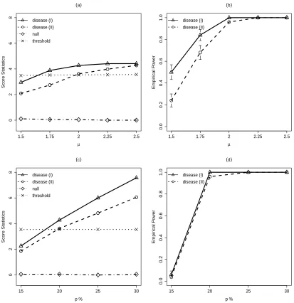
We first examine the effects of CNV jump sizeµon the CNVtest performances where

the CNV carrier frequency is fixed at 20% in cases and 10% in controls for the

disease-associated CNVs, and at 15% in both cases and controls for the null CNV. Figure

2.1 (a) shows the score statistics calculated for the null CNV and also the

disease-associated CNVs with the jump size changing from 1.5 to 2.5, together with the

threshold level determined by (2.9). We observe that the score statistics for the null

CNV is constant and is always much smaller than the threshold. On the other hand,

the score statistics for the disease associated CNVs increases asµincreases. In

addi-tion, shifts in exact CNV boundaries lead to smaller score statistics, especially when

µ is small. Figure 2.1 (b) shows the empirical power of CNVtest for identifying the

(31)

the true CNVs. Again, shifts in exact CNV boundaries lead to a slight loss of power,

especially whenµis small. We observed that the empirical over-selections are always

zero for all data sets simulated, and they are not affected by the values of µ.

We then fixµ= 2.0 and examine how the carrier proportion in cases affects the power

of identifying the disease-associated CNVs. Figure 2.1 (c) shows the score statistics

evaluated for the null CNV and the disease-associated CNVs with carrier proportion

in cases changing from 15% to 30%, together with the threshold level determined

by (2.9). We observe that the score statistics for the null CNV are constant and

always much smaller than the threshold. On the other hand, the score statistics for

the disease associated CNVs increase as the carrier proportion in the cases increases.

Again, for all simulations, we did not observe any false identification.

2.5. Application to Population Differentiation CNV study

Redon et al. (2006) presented the first genome-wide global variation analysis of DNA

copy number in the human genome where DNA EBV-transformed lymphoblastoid

cell lines of the 270 HapMap samples was screened for CNVs using clone-based

com-parative genomic hybridization (Whole Genome TilePath, WGTP) array consisting

of 26,463 large-insert clones. To demonstrate our method, we consider data from

two populations: 89 of European descent from Utah (CEU), 45 unrelated Japanese

from Tokyo (JPT) and 45 unrelated Han Chinese from Beijing (CHB). Our goal is to

identify the genomic regions that show difference in copy number between CEU and

Asian populations (JPT+CHB). Such population differentiation in CNV can provide

important insights into genetic diversity and evolution.

For each individual, we first standardize the clone intensity data by mean and variance

calculated for this individual. Since one clone covers a longer region than the SNP

(32)

(a) µ Score Statistics disease (I) disease (II) null threshold 0 2 4 6 8

1.5 1.75 2 2.25 2.5

(b)

µ Empir ical P o w er disease (I) disease (II) 0.0 0.2 0.4 0.6 0.8 1.0

1.5 1.75 2 2.25 2.5

(c)

p % Score Statistics disease (I) disease (II) null threshold 0 2 4 6 8

15 20 25 30

(d)

p % Empir ical P o w er disease (I) disease (II) 0.0 0.2 0.4 0.6 0.8 1.0

15 20 25 30

Figure 2.1: Simulation results. (a)-(b): Effect of the CNV jump size µ from 1.5

to 2.25 on (a) score statistics for CNVs with carrier probability of 20% in case and

10% in control and (b) power of detecting the associated CNV. (c)-(d): Effect of

the CNV frequency in case p from 15% to 30% on (c) score statistics for CNVs with

carrier probability of 20% in case and 10% in control and (d) power of detecting the associated CNV.

data, we choose L = 10 in our CNVtest so that the largest CNV covers at most 10

clones. Here we consider both duplication and deletion copy number variants and

(33)

deletion, where ν = p

2 log(mL) _≈ 4.997. The resulting ˆrdup₍₌ _|Rdup_|_{) = 26}_,₄₉₆

and ˆrdel₍₌ _|Rdel_|_{) = 13}_,_{585. Note that both ˆ}_rdup _{and ˆ}_rdel _{are much smaller than}

the number of possible intervals in the whole genome, which is at the order of m2_.

Consequently, the threshold λdup ₌p

2 log(ˆrdup₎ _≈ ₄_._{513 and} _λdel ₌ p

2 log(ˆrdel₎ _≈

4.363, respectively.

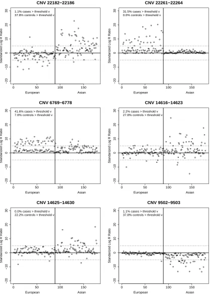
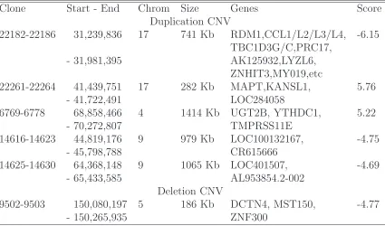
CNVtest identified five duplication CNVs and one deletion CNV that showed different

frequencies between the European and Asian populations. Table 2.1 shows their clone

locations, size, overlapping genes and their score statistics defined in (2.8). Figure

2.2 shows the scatter-plots of the length-adjusted sum of clone intensity statistics

defined in (2.2) for each of the samples for each of the six identified CNV regions,

clearly indicating the differences of the carrier frequencies. To show that the clones

in the identified CNV regions indeed have different intensities for samples in these

two different populations, we present in Figure 2.3 the observed clone intensities for

the clones within and outside the identified CNV regions respectively for each of the

samples. Again, the identified CNV regions indeed show some differences in clone

intensities from their neighboring clones. Note that the two CNVs on chromosome

9 are very close to each other and have similar intensity patterns in the samples. It

is likely that they form a large CNV. This is due to the fact that we chose L = 10

in CNVtest. However, as in any CNV analysis, a post-processing step may simply

combine these two CNVs into one.

Redon et al. (2006) reported two CNVs that exhibit the highest population

differen-tiation between CEU and JPT+CHB, one of which, the duplication CNV on

chro-mosomes 17 that includes gene MAPT, is also identified by CNVtest. CNVtest did

not identify the CNV on chromosome 3 reported by Redon et al. (2006). However,

this CNV only includes one clone and does not have any known genes in it. The

(34)

deletion CNV identified by CNVtest, which includes gene DCTN4, was presented to

have the highest population differentiation between CEU and Yoruban samples. The

intensity plot in Figure 2.3 for this region shows clear a difference between the CEU

and JPT+CHB samples.

Besides samples from CEU and JPT+HCB, Redon et al. (2006) also obtained the

clone data for 90 Yoruban (YRI) samples. When comparing CEU and YRI, CNVtest

identified 4 deletion CNVs and 11 duplication CNVs that showed very different

fre-quencies. These CNVs include all 6 CNVs that were reported in Redon et al. (2006)

to have the highest population differentiation. When comparing YRI and JPT+HCB,

CNVtest identified 2 deletion CNVs and 12 duplication CNVs, including 2 CNVs that

were reported in Redon et al. (2006) to have the highest population differentiation.

2.6. Conclusion and Discussion

We have developed a new statistical method, CNVtest, for genome-wide CNV

asso-ciation studies. Compared with the commonly used two-step approaches, CNVtest

is computationally much faster because the genome is only scanned once. The

com-putational complexity of this method is the same as the likelihood ratio selector of

Jeng et al. (2010) and the multiple sample CNV analysis procedure of Jeng et al.

(2013), all in the order of O(mL). In addition, it avoids the often troublesome task

of determining which CNV regions one should test for association and how to adjust

for multiple comparisons. The method is particularly effective when the CNV regions

from the different carriers do not exactly cover the same intervals. The CNVtest is

also flexible and can be applied to identify CNVs associated with different phenotypes

through the use of the generalized linear models.

(35)

0 50 100 150 −20 −10 0 10 20

30 1.1% cases > threshold v

37.8% controls > threshold v

CNV 22182−22186

European Asian

Standar

iz

ed Log R Ratio

0 50 100 150

−20

−10

0

10

20

CNV 22261−22264

European Asian

Standar

iz

ed Log R Ratio

0 50 100 150

−20

−10

0

10

20

CNV 6769−6778

European Asian

Standar

iz

ed Log R Ratio

0 50 100 150

−20

−10

0

10

20

CNV 14616−14623

European Asian

Standar

iz

ed Log R Ratio

0 50 100 150

−20

−10

0

10

20

CNV 14625−14630

European Asian

Standar

iz

ed Log R Ratio

0 50 100 150

−20

−10

0

10

20

CNV 9502−9503

European Asian

Standar

iz

ed Log R Ratio

(36)

22175 22190 20 40 60 80 −15 −10 −5 0 5 10 15 CNV 22182−22186 European 22175 22190 20 40 60 80 −15 −10 −5 0 5 10 15 CNV 22182−22186 Asian 22255 22270 20 40 60 80 −20 −10 0 10 20 CNV 22261−22264 European 22255 22270 20 40 60 80 −20 −10 0 10 20 CNV 22261−22264 Asian 6760 6775 20 40 60 80 −15 −10 −5 0 5 10 15 CNV 6769−6778 European 6760 6775 20 40 60 80 −15 −10 −5 0 5 10 15 CNV 6769−6778 Asian 14610 14625 20 40 60 80 −15 −10 −5 0 5 10 15 CNV 14616−14623 European 14610 14625 20 40 60 80 −15 −10 −5 0 5 10 15 CNV 14616−14623 Asian 14615 14630 20 40 60 80 −10 −5 0 5 10 CNV 14625−14630 European 14615 14630 20 40 60 80 −10 −5 0 5 10 CNV 14625−14630 Asian 9495 9505 20 40 60 80 −10 −5 0 5 10 CNV 9502−9503 European 9495 9505 20 40 60 80 −10 −5 0 5 10 CNV 9502−9503 Asian

(37)

Table 2.1: The CNVs identified by CNVtest that show different frequencies between Europe and Asian populations. Clone locations, chromosome, CNV size, overlapping genes (based on NCBI36, March 2006, Build 19) and the corresponding score statistics (Score) are shown.

Clone Start - End Chrom Size Genes Score

Duplication CNV

22182-22186 31,239,836 17 741 Kb RDM1,CCL1/L2/L3/L4, -6.15

TBC1D3G/C,PRC17,

- 31,981,395 AK125932,LYZL6,

ZNHIT3,MY019,etc

22261-22264 41,439,751 17 282 Kb MAPT,KANSL1, 5.76

- 41,722,491 LOC284058

6769-6778 68,858,466 4 1414 Kb UGT2B, YTHDC1, 5.22

- 70,272,807 TMPRSS11E

14616-14623 44,819,176 9 979 Kb LOC100132167, -4.75

- 45,798,788 CR615666

14625-14630 64,368,148 9 1065 Kb LOC401507, -4.69

- 65,433,585 AL953854.2-002

Deletion CNV

9502-9503 150,080,197 5 186 Kb DCTN4, MST150, -4.77

- 150,265,935 ZNF300

the next generation sequencing. One can use the local median transformation

proce-dure proposed in Cai et al. (2012) to transform the read-depth data to approximately

normally distributed data and directly apply the CNVtest to the transformed data.

We expect to have similar power and genome-wide error control as the intensity-based

data.

(38)

CHAPTER 3 Kernel-based Tests for Two-sample Differential

Enrichment Analysis Using ChIP-seq data

3.1. Introduction

Chromatin immunoprecipitation sequencing (ChIP-seq) technology is a powerful tool

for analyzing protein interactions with DNA (Park, 2009). ChIP-seq combines

chro-matin immunoprecipitation (ChIP) with massively parallel DNA sequencing to

iden-tify the binding sites of DNA-associated proteins. It can be used to map global

binding sites of transcription factors (TFs) and genomic landscape of histone

modi-fication marks (HMs). This high-throughput technology can create millions of short

parallel sequencing reads and provide more accurate mapping information for the

binding regions in the whole genome with lower cost (Johnson et al., 2007; Mikkelsen

et al., 2010; Mortazavi et al., 2008; Barski et al., 2007) than array-based methods.

Both TF binding and histone modification play important roles in gene regulation,

where TFs bind to DNA at a promoter region to promote or block gene transcription.

The signal of TFs usually shows one sharp peak at binding sites. Multiple histone

modification marks have been reported to be associated with transcription

initial-ization, open chromatin and repression of transcription (Mikkelsen et al., 2010; Hon

et al., 2009).

Most previous work in analysis of ChIP-seq data has focused on developing

peak-calling procedures to find the binding sites for TFs (Zhang et al., 2008b; Kuan et al.,

2011; Ji et al., 2008; Schwartzman et al., 2013; Spyrou et al., 2009). Identifying the

(39)

spread out (O’Geen et al., 2011). The signals of HMs are diffuse and usually have

multiple local peaks, which are hard to identify by directly applying peak-calling

algorithms.

Another important question is to identify the genomic regions that show differential

enrichment of histone modification between two experimental conditions, such as

dif-ferent cellular states or difdif-ferent time points (Mikkelsen et al., 2010; Liang and Kele¸s,

2012). Indeed, different types of differential enrichment have been observed,

includ-ing shift of nucleosome positions, peak height differences and presence/absence of HM

marks (Chen et al., 2011; He et al., 2010). Chen et al. (2011) further demonstrated

that the spatial distributions of histone marks are predictive for promoter locations

and promoter usage. Angel et al. (2011) show that during cold, the H3K27me3 levels

progressively increase at a tightly localized nucleation region in Arabidopsis,

indi-cating the importance of studying the peak height, not just the presence/absence of

peaks.

One common approach to identifying differentially enriched regions is to apply a

peak-calling algorithm to identify the enriched regions for each of the two conditions.

The regions with peaks in one condition but without peaks in the other condition are

then selected. However, selection of enriched regions often depends on the thresholds

used in the peak-calling algorithm. Small differences in the calculated p-values or the

FDR threshold used by the peak-finding program can lead to very different sets of

peaks. Furthermore, this simple procedure has limitations in detecting the differential

enrichment of different peak heights or different peak locations.

Several parametric methods based on Poisson/negative binomial distribution have

been proposed to address this differential enrichment problem in ChIP-seq data such

as DiffBind and DBChIP (Stark and Brown, 2011; Liang and Kele¸s, 2012). Most of

(40)

these methods require biological replications to estimate the parameters, especially

the dispersion parameter in the negative binomial model (Kuan et al., 2011). However,

many ChIP-seq data usually have a few or even no replicates. Taslim et al. (2009)

proposed a nonlinear method that uses locally weighted regression (Lowess) for

ChIP-seq data normalization. Shao et al. (2012) developed a method to quantitatively

compare ChIP-seq data sets. To circumvent the issue of differences in signal-to-noise

ratios between samples, they focused on ChIP-enriched regions and introduced the

idea that ChIP-seq common peaks could serve as a reference to build the rescaling

model for normalization. The inputs of all the methods mentioned rely on first

identifying the enriched regions and then obtaining the total tag or read counts in

these regions. Such approaches have two limitations. First, one has to identify the

regions using peak-finding algorithms. Second, by summarizing the number of tags

into one single number of the region, one can potentially lose important spatial profile

differences such as shifts of the signal region or shapes of signals.

In this Chapter , we propose a nonparametric method to identify the genes with

differentially enriched regions based on the ChIP-seq data. Instead of first identifying

the enriched regions or peaks as most of the existing methods do, we consider the

regions close to genes that may contain important regulatory elements such as the

promoter regions, the gene body and downstream regions of the genes. For each

of the regions, we summarize the data as counts of sequencing reads in each of the

bins of a given length (e.g., 25 bps). The counts in these candidate regions provide

important information about different HM levels between two cellular states. After

transforming the count data to approximately normal, we apply kernel smoothing to

the differences of the data and develop a nonparametric hypothesis testing based on

(41)

local differences that are unlikely to be biologically relevant.

We demonstrate the method using ChIP-seq data on a comparative epigenomic

pro-filing of adipogenesis of murine 3T3-L1 cells reported in Mikkelsen et al. (2010). Our

method detects genes with differential H3K27ac levels at gene promoter regions

be-tween proliferating preadipocytes and mature adipocytes, which agree with what were

observed in Mikkelsen et al. (2010) based on fold-change analysis. The test

statis-tics also correlate with the gene expression changes well, indicating that the identified

differences are indeed biologically meaningful. Our results also indicate that the

com-bination of different histone modification profiles can predict the fold changes of gene

expressions very well.

3.2. A Motivating Comparative ChIP-seq Study, Data Transformation

and Statistical Model

We consider the ChIP-seq experiments reported in Mikkelsen et al. (2010) on murine

3T3-L1 cells undergoing adipogenesis. Specifically, they generated genome-wide

chro-matin state maps using ChIP-seq profiling, where they mapped six HMs and two TFs

at four time points, including proliferating (day -2) and confluent (day 0) preadipocytes,

immature adpipocytes (day 2) and mature adipocytes (day 7). We focus our

anal-ysis on H3K27ac mark, which is expected to be enriched at active promoters or

enhancers. In order to identify the genes that show differential H3K27ac levels

be-tween the preadipocytes (day -2) and mature adipocytes (day 7), we consider the

upstream 5000 bp region and downstream 2000 bp regions around transcription start

site (TSS) for each gene and divide the regions into 280 bins of 25bps. We map the

raw data using Bowtie (Langmead et al., 2009), extend reads to the fragment size

and then obtain the genome wide coverage data with a fixed bin size of 25 bp. Since

(42)

the two ChIP-seq samples usually are sequenced at different depths (total number of

reads). We scale the counts according to the sequencing depth ratio. Suppose that

there are m genes and for each gene i, there are n observed read counts Xikj in bin

k under condition j, for i = 1,_{· · ·} , m, k = 1,_{· · ·} , n and j = 1,2. Our goal is to find

the genes with differential H3K27ac levels at their promotor regions between mature

adipocytes and preadipocytes.

For each gene i and each condition j, we assume the data Xikj, k = 1,· · · , n are

ap-proximately Poisson with meansµikj. We first apply variance-stabilizing

transforma-tion (VST) procedure to transform the variables to the variablesX∗

ikj = 2

p

Xikj + 0.25,

as recommended by Brown et al. (2010, 2005). Thus, we can treatX∗

ikj’s as

approxi-mate normal variables with mean 2p

λikj and variance of 1. For theith gene, in order

to test for differential enrichment between two conditions, we calculate the difference

between the two conditions asYik =Xik1∗ −Xik2∗ . If there is no differential enrichment,

YT

i = (Yik, ..., Yin) should have a mean value of zero.

We further denote Yi(tk) = Yik, for tk = k/n ∈ (0,1], k = 1, ...., n. We assume the

following “signal+white noise” model for the normalized differences,

Yi(tk) =fi(tk) +σiWi(tk), (3.1)

where fi(t) is a smooth function that characterizes the difference of the ChIP-seq

enrichment profiles and Wi(tk) is Gaussian noise with mean 0 and variance 1. For

the ith gene, the null hypothesis that there is no differential enrichment between two

conditions is equivalent to testing

(43)

3.3. Kernel-smoothing-based Nonparametric Tests

For a given gene i, we propose a kernel-smoothing based nonparametric test (Lepski

and Spokoiny, 1999) to test the null hypothesis (3.2). For notational simplicity,

we omit the subscript i in the following. Let K be a proper kernel, which is a

symmetric, continuous density function with expectation zero. We use a normal

kernel function, which satisfies all these regularity conditions and fits the real data

well. For a fixed bandwidth value λ ∈ [0,1], we consider the kernel estimator ˜Yλ(t)

with t∈[0,1],s ∈[0,1] and its standard decomposition as

˜

Yλ(t) =

1

λ Z

K

t₋s λ

Y(s)ds (3.3)

= 1

λ Z

K

t₋s λ

f(s)ds+σ

λ Z

K

t₋s λ

W(s)ds

= fλ(t) +σξλ(t)

where fλ(t) = 1_λ

R

K(t−s

λ )f(s)ds and ξλ(t) = 1 λ

R

K(t−s

λ )W(s)ds.

Based on Lepski and Spokoiny (1999), we use the integral of the squared kernel

estimator Tλ defined as

Tλ = ||

˜

Yλ||2

ˆ

σ2 =

R1

0 Y˜

2 λ(t)dt

ˆ

σ2 (3.4)

to test the null hypothesis H0 : ||f(t)|| = 0, where ˆσ2 is some estimate of the error

variance, which we discuss in Section 3.3.2. Under the null H0, one has

˜

Y0λ(t) =σξλ(t) (3.5)

(44)

and the test statistic becomesT0λ =

R1

0 ξ

2

λ(t)dt. Since W(ti) follows N(0,1), we have

ξλ(t) =

1

λ Z 1

0

K

t₋s λ

W(s)ds

For the Gaussian kernel, the expectation of T0λ is given by

E(T0λ) =

1

nλ||K||

2 ₌ 1

nλ

1 2√π.

We derived the closed-form variance as

Var(T0λ) =

1

n2_λ

1

√

2π.

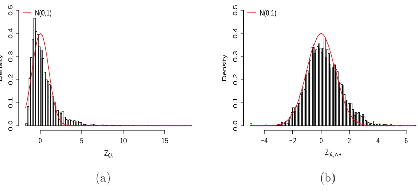
(see Appendix B.1 for derivation). We can then define the test statistic as

Z0λ =

Tλ−E(T0λ)

p

Var(T0λ)

, (3.6)

which follows N(0,1) as n → ∞under the null hypothesis.

3.3.1. An alternative derivation of the test statistic

We present in this section an alternative derivation of the test statistic that has better

finite sample performance than the statistic (3.6) whenn is not too large (see Section

3.4 for an illustration). Note that the kernel smoother ˜Yλ(t) can be written as a linear

combination of YT _{= (}_Y

1, ..., Yn),

˜

(45)

where Sλ is considered as the hat matrix,

Sλ =

1 nλ      

K(t1−s1

λ ) . . . K( t1−sn

λ )

... . .. ...

K(tn−s₁

λ ) . . . K( tn−sn

λ )       .

and the trace of Sλ is the degrees of freedom (df) of the kernel smoother (Hastie and

Tibshirani, 1990).

Based on (3.3), (3.4) and (3.7), the statisticTλ can be approximated by

Tλ =

1 nσ2 n X k=1 ˜ Yk 2 λ = 1

nσ2Y T

ST

λSλY (3.8)

where the n_×n matrix ST

λ is the transpose ofSλ. Let M =SλTSλ with the following

eigen-decomposition, VT_{M V} ₌ _D, _where _D ₌ _diag₍_d

1, ..., dn), d1 ≥ ... ≥ dn, are

the eigenvalues and V is the orthogonal matrix of the eigenvectors. Under the null,

based on (3.5), Y /σ follows a multivariate normal distribution Nn(0, In). Let UT =

(U1, ..., Un) =VTY /σ, we can rewrite Tλ as

Tλ =

1

nU

T

DU = 1

n

X

k=1

dkUk2.

Since V is an orthogonal matrix, under the null hypothesis, the vector U follows

Nn(0, V VT) =Nn(0, In) and therefore Uk2 are i.i.drandom variables followingχ21 and

Tλ follows a mixture ofn χ2 distributions with weights dk/n. Furthermore, based on

Bentler and Xie (2000), under the null, Tλ can be approximated by a weighted χ2

distribution, δχ2

d, where

d=⌈(

n

X

k=1

dk)2/ n

X

k=1

d2_k⌉, δ=

n

X

k=1

dk/n

/d.

(46)

Alternatively, using the Wilson-Hilferty transformation (Wilson and Hilferty, 1931),

we have

Z0λ,W H =

3

q

Tλ

δd −

1− 2

9d

q

2 9d

, (3.9)

which follows aN(0,1) under the null hypothesis (see Appendix B.2 for details). We

use this statistic in our analysis.

3.3.2. Estimate σ for each gene

In order to calculate the test statistic specified as (3.4) or (3.8), we need the variance

estimate ˆσi2 for each gene i. After the transformation steps in Section 3.2, for each

gene i, we assume that the observations Yik have the same varianceσi2. We consider

the Nadaraya-Watson nonparametric regression with kernel smoothers as (3.3),

˜

Yλ(t) = SλY

where df = tr(Sλ) is the degrees of freedom of the kernel smoother (Hastie and

Tibshirani, 1990). We can estimate the variance σ2

i by calculating the residual sum

of squares

ˆ

σ2 = [ ˜Yλ(t)−Y(t)]

T_{[ ˜}_Y

λ(t)−Y(t)]

n₋df =

Pn

k=1[Yk−Y˜λ(tk)]2

n₋df . (3.10)

Since we consider the ChIP-seq data with very few or no replications, the estimates

ˆ

σ2

i can be too small for very small counts. To improve precision, we use an approach

similar to Efron et al. (2001) and Tusher et al. (2001): we add a constant a0 = 90th

Statistical Methods for Analysis of Multi-Sample Copy Number Variants and ChIP-seq Data

University of Pennsylvania

ScholarlyCommons

Statistical Methods for Analysis of Multi-Sample

Copy Number Variants and ChIP-seq Data

Qian Wu

Statistical Methods for Analysis of Multi-Sample Copy Number Variants

and ChIP-seq Data

ACKNOWLEDGEMENT

ABSTRACT

TABLE OF CONTENTS

LIST OF TABLES

LIST OF ILLUSTRATIONS

CHAPTER 1

Introduction

1.1. Copy Number Variants

1.2. ChIP-seq Experiments

CHAPTER 2

A Statistical Method for detecting trait-associated

Copy Number Variants

2.1. Introduction

2.2. Statistical Model and CNV Association Test

2.3. A Procedure for Identifying the Trait-associated CNVs and Its

Theoretical Properties

2.4. Simulation Studies

2.5. Application to Population Differentiation CNV study

2.6. Conclusion and Discussion

CHAPTER 3

Kernel-based Tests for Two-sample Differential

Enrichment Analysis Using ChIP-seq data

3.1. Introduction

3.2. A Motivating Comparative ChIP-seq Study, Data Transformation

and Statistical Model

3.3. Kernel-smoothing-based Nonparametric Tests