University of Pennsylvania
ScholarlyCommons
Publicly Accessible Penn Dissertations
1-1-2014
Estimation and Inference of the Three-Level
Intraclass Correlation Coefficient
Matthew David Davis
University of Pennsylvania, [email protected]
Follow this and additional works at:http://repository.upenn.edu/edissertations
Part of theBiostatistics Commons
This paper is posted at ScholarlyCommons.http://repository.upenn.edu/edissertations/1252 For more information, please [email protected].
Recommended Citation
Davis, Matthew David, "Estimation and Inference of the Three-Level Intraclass Correlation Coefficient" (2014).Publicly Accessible
Penn Dissertations. 1252.
Estimation and Inference of the Three-Level Intraclass Correlation
Coefficient
Abstract
Since the early 1900's, the intraclass correlation coefficient (ICC) has been used to quantify the level of agreement among different assessments on the same object. By comparing the level of variability that exists within subjects to the overall error, a measure of the agreement among the different assessments can be calculated. Historically, this has been performed using subject as the only random effect. However, there are many cases where other nested effects, such as site, should be controlled for when calculating the ICC to determine the chance corrected agreement adjusted for other nested factors. We will present a unified framework to estimate both the two-level and three-level ICC for both binomial and multinomial outcomes. In addition, the corresponding standard errors and confidence intervals for both ICC measurements will be displayed. Finally, an example of the effect that controlling for site can have on ICC measures will be presented for subjects nested within genotyping plates comparing genetically determined race to patient reported race.
In addition, when determining agreement on a multinomial response, the question of homogeneity of agreement of individual categories within the multinomial response is raised. One such scenario is the GO project at the University of Pennsylvania where subjects ages 8-21 were asked to rate a series of actors' faces as happy, sad, angry, fearful or neutral. Methods exist to quantify overall agreement among the five responses, but only if the ICCs for each item-wise response are homogeneous. We will present a method to determine homogeneity of ICCs of the item-wise responses across a multinomial outcome and provide simulation results that demonstrate strong control of the type I error rate. This method will subsequently be extended to verify the assumptions of homogeneity of ICCs in the multinomial nested-level model to determine if the overall nested-level ICC is sufficient to describe the nested-level agreement.
Degree Type
Dissertation
Degree Name
Doctor of Philosophy (PhD)
Graduate Group
Epidemiology & Biostatistics
First Advisor
Warren B. Bilker
Second Advisor
J. Richard Landis
Keywords
Subject Categories
ESTIMATION AND INFERENCE OF THE THREE-LEVEL INTRACLASS CORRELATION COEFFICIENT
Matthew Davis
A DISSERTATION
in
Epidemiology and Biostatistics
Presented to the Faculties of the University of Pennsylvania
in
Partial Fulfillment of the Requirements for the
Degree of Doctor of Philosophy
2014
Supervisor of Dissertation Co-Supervisor of Dissertation
Warren B. Bilker J. Richard Landis
Professor of Biostatistics Professor of Biostatistics
Graduate Group Chairperson
John H. Holmes, Associate Professor of Medical Informatics in Epidemiology
Dissertation Committee
Sharon Xiangwen Xie, Associate Professor of Biostatistics
ESTIMATION AND INFERENCE OF THE THREE-LEVEL INTRACLASS CORRELATION COEFFICIENT
c
COPYRIGHT
2014
Matthew Davis
This work is licensed under the Creative Commons Attribution NonCommercial-ShareAlike 3.0
License
To view a copy of this license, visit
ACKNOWLEDGEMENT
First, I would like to thank God for providing me the strength, fortitude and perse-verance to undertake this endeavor and see it to completion.
Worthy are you, our Lord and God, to receive glory and honor and power, for you created all things, and by your will they existed and were created. -Revelation 4:11
I would like to thank Dr. Warren Bilker for his unending support of my dissertation. The time, energy and care Dr. Bilker put towards this dissertation went beyond what was necessary, and this work would not have been possible without his guidance. I would also like to thank Dr. J. Richard Landis for overseeing our work, from providing the original dissertation research question to providing careful input and oversight throughout the life of the project. I am grateful to my committee members, Dr. Sharon Xie and Dr. Robert DeRubeis, for providing helpful feedback on this research. In addition, I am grateful to Carla Hultman, Pat Spann, Marissa Fox and Catherine Vallejo for their invaluable organizational support. I would also like to thank Dr. Benjamin French for overseeing my master’s thesis and for his guidance through that process. Finally, I would like to acknowledge all of the faculty and staff of the Department of Biostatistics and Epidemiology for their unending support of my work at the University of Pennsylvania.
ABSTRACT
ESTIMATION AND INFERENCE OF THE THREE-LEVEL INTRACLASS CORRELATION COEFFICIENT
Matthew Davis
Warren B. Bilker
J. Richard Landis
Since the early 1900s, the intraclass correlation coefficient (ICC) has been used to quantify the level of agreement among different assessments on the same object. By comparing the level of variability that exists within subjects to the overall error, a measure of the agreement among the different assessments can be calculated. His-torically, this has been performed using subject as the only random effect. However, there are many cases where other nested effects, such as site, should be controlled for when calculating the ICC to determine the chance corrected agreement adjusted for other nested factors. We will present a unified framework to estimate both the two-level and three-two-level ICC for both binomial and multinomial outcomes. In addition, the corresponding standard errors and confidence intervals for both ICC measure-ments will be displayed. Finally, an example of the effect that controlling for site can have on ICC measures will be presented for subjects nested within genotyping plates comparing genetically determined race to patient reported race.
TABLE OF CONTENTS
ACKNOWLEDGEMENT . . . iii
ABSTRACT . . . v
LIST OF TABLES . . . ix
LIST OF ILLUSTRATIONS . . . x
CHAPTER 1 : Introduction . . . 1
1.1 Introduction to Measures of Agreement . . . 1
1.2 Estimation and Inference of the Three-Level Intraclass Correlation Co-efficient . . . 13
CHAPTER 2 : A Test of Homogeneity of Dependent Intraclass Correlation Coefficients for Multinomial Data . . 15
2.1 Introduction . . . 15
2.2 Notation and Motivation . . . 17
2.3 Distributions for Overdispersed Multinomial Data . . . 17
2.4 Homogeneity of ICCs . . . 22
2.5 Simulations . . . 27
2.6 Applications . . . 32
2.7 Conclusion . . . 34
3.2 Notation and Motivation . . . 39
3.3 Obtaining the Variance of xi·. . . 45
3.4 Current ICC Methods . . . 47
3.5 The Nested-Level ICC . . . 50
3.6 Simulations . . . 56
3.7 Nested-Level Agreement in a GWAS . . . 61
3.8 Immediate Extension . . . 64
3.9 Conclusion . . . 64
CHAPTER 4 : On the Nested-Level Intraclass Correlation Coef-ficient for Multinomial Data . . . 66
4.1 Introduction . . . 66
4.2 Notation . . . 67
4.3 Distributions for Overdispersed Multinomial Data . . . 68
4.4 Goodness-of-Fit Testing . . . 74
4.5 Application: ”Fingerprinting” within a GWAS . . . 79
4.6 Conclusion . . . 86
CHAPTER 5 : Discussion . . . 87
APPENDICES . . . 90
LIST OF TABLES
TABLE 1.1 : Interpretation of ICC Measures from Landis and Koch (1977a) 5
TABLE 2.1 : Power of Homogeneity of ICC Test . . . 30 TABLE 2.2 : Application Results . . . 34
TABLE 3.1 : Agreement between Self-Reported and Genetically-Inferred Eth-nicity . . . 40 TABLE 3.2 : Levels of Agreement among Race Responses in a GWAS . . . 42 TABLE 3.3 : Simulation Results for π = 0.3 . . . 59 TABLE 3.4 : Simulation Results for π = 0.5 . . . 60 TABLE 3.5 : Levels of Agreement among Ethnicity Responses in a GWAS
Reanalyzed . . . 62
LIST OF ILLUSTRATIONS
CHAPTER 1
Introduction
”It is by universal misunderstanding that all agree. For if, by ill luck, people un-derstood each other, they would never agree.” Little did Charles Baudelaire know that his penned words 150 years prior would be a fitting description for statistical studies on methods of agreement. Given multiple ratings on the same object, it is a result of naivety that one would think that all raters would agree in their inter-pretation of the object. In addition, according to Mr. Baudelaire, even if the raters were lucky enough to fully understand one another’s way of thinking, they still would not agree on the individual assessments on the objects. As a result, it is necessary to study statistical measures of agreement to better quantify how well independent raters agree when assessing the same object. This dissertation reviews the scope of available published work on measures of agreement and will add to these measures in two areas. First, a test for homogeneity of intraclass correlation coefficients (ICCs) will be derived across separate responses within a multinomial outcome. Second, the concept of a nested-level of agreement will be examined, and methods for estimat-ing and providestimat-ing inference on the nested-level agreement will be presented for both binary and multinomial outcomes.
1.1. Introduction to Measures of Agreement
coef-ficient of variation, dichotomous outcomes and multiple raters and categories. The summary of methods of agreement for kappa statistics and the intraclass correlation coefficients are of particular interest and provide an important summary of available methods that are directly applicable to this research. While this dissertation focuses mainly on the methods summarized by Shoukri, the following references are provided to more completely describe the current status of the methods of measures of agree-ment. Analyzing Rater Agreement: Manifest Variable Methods[49] by Von Eye and Mun provides a framework to assess rater agreement based on log-linear models. In
Statistical Tools for Measuring Rater Agreement, Lin et. al.[36] examine methods of rater agreement using the concordance correlation coefficient (CCC) as a basis. In this book, agreement methods for both continuous and categorical data are developed and corresponding power and sample size methods are presented. Lastly, Broemeling provides a Bayesian description of measures of agreement in Bayesian methods for measures of agreement[7] focusing both categorical and continuous outcomes.
1.1.1. Kappa Statistic
The kappa statistic was originally proposed by Cohen (1960)[13] as a chance corrected measure of agreement between two raters and is calculated as
ˆ
κ= Po−Pe 1−Pe
(1.1)
where Po is the observed proportion of agreement between the two raters and Pe is
the expected measure of agreement by chance. ˆκhas limits [−Pe
1−Pe,1] depending on the
observed level of agreement. Regarding estimation of a standard error of the kappa statistic, Fleiss, Nee and Landis (1979)[23] wrote ”Many human endeavors have been cursed with repeated failures before final success. The scaling of Mount Everest is one example. The discovery of the Northwest Passage is a second. The derivation of a correct standard error for kappa is a third!” A closed-form solution for the exact variance of ˆκ has not yet been discovered, however an asymptotic variance can be found in Fleiss et. al. (1979)[23]. While ˆκ is commonly used to quantify measures of agreement among raters, it is only applicable in situations where there are only two raters and a binomial response, necessitating further methods that can handle more diverse cases.
1.1.2. Weighted Kappa Statistic
The weighted kappa statistic was developed 8 years after the original kappa statistic by Cohen (1968)[14], which allows for a measure of agreement for a multinomial outcome based on a set of weights. For k possible outcomes, a k ×k contingency table can be constructed for each possible combination of ratings for two ratings on the same object, and let i and j index the cell for responses i from rater 1 and j
observed probability of response for cell (i, j) and peij be the expected probability of
response for cell (i, j). Then the weighted kappa statistic can be calculated as
κw = 1−
P
vijpoij
P
vijpeij
(1.2)
The weighted kappa statistics allows for researchers to specify weights for the analysis giving stronger weights towards specific levels of agreement, allowing for customizable measures of agreement for a given response. Interestingly, using the weights vij =
(i−j)2, Fleiss and Cohen (1973)[21] proved that the resulting weighted kappa statistic is equivalent to the intraclass correlation coefficient, drawing a direct comparison between the two measures of agreement. Krippendorff (1970)[30] showed a similar result. The remainder of measures of agreement to be covered will focus on the ICC, however the concept of chance corrected agreement will be important to developing an adjusted nested-level ICC estimate.
1.1.3. Intraclass Correlation Coefficient
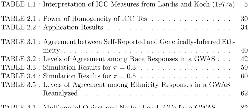
The intraclass correlation coefficient was first introduced by J. Arthur Harris in 1913 [25] as a measurement of agreement for multiple ratings on the same object. Since its inception, the volume of literature describing and implementing the ICC has grown exponentially. Originally intended for continuous outcomes, the ICC was expanded to describe rater agreement for categorical data as well by Landis et. al. (1977) [33, 34], Fleiss and Cohen (1973)[21] and Krippendorff (1970)[30]. In addition, at this time rules of thumb for interpretation of the ICC were given by Landis and Koch (1977a)[33] that assisted in quantifying the ICC.
Table 1.1: Interpretation of ICC Measures from Landis and Koch (1977a)
Kappa Statistic Strength of Agreement
<0.00 Poor
0.00-0.20 Slight 0.21-0.40 Fair 0.41-0.60 Moderate 0.61-0.80 Substantial 0.81-1.00 Almost Perfect
of the ICC as a measure of agreement for categorical outcomes. By 1999, Ridout et. al. [44] documented and compared 20 distinct methods for estimating the ICC for binomial data. For the purposes of this research, we will focus on two methods of calculating and providing inference on the ICC, the components of variance model introduced by Landis and Koch (1977c) [34] and the beta-binomial estimate of the ICC introduced by Crowder (1978, 1979) [15, 16].
Components of Variance Model
ANOVA methods of determining the ICC were documented by numerous researchers including Anderson and Bancroft [1], Scheff´e [45] and Searle [46], however flexible models to handle varying number of raters per object did not arise until Landis and Koch [34] presented the variance components approach for estimating the ICC. According to their approach, the binomial response yij for object i and rater j can
be modeled by
yij =µ+si+eij (1.3)
where µ is the overall probability of response yij = 1, si are normally distributed
errors with mean 0 and varianceσs2 andeij are normally distributed errors with mean
the between-subject variance categorized as σ2
s. The corresponding ICC is calculated
as
ρ= σ
2
s
σ2
s +σe2
(1.4)
as the ratio of the variance attributed to the between-subject error and the total variance. Therefore, larger ICC values would indicate that the overall variability is dominated by the between-subject error and not the within-subject error attributed to multiple ratings on an object, indicating that the raters in the model exhibit a high level of agreement on the objects they are rating. Landis and Koch extended this model to account for multinomial data and provided an asymptotic standard error calculation that involved the use of complex matrix calculations as described in Koch et. al. (1977) [29]. Further improvements on the standard error calculations were made, such as the development of more computationally simple variance for the ICC published by Mak (1988)[39] that relies on fewer assumptions than the Landis and Koch calculations. However, as these improvements are not needed for the research presented in this dissertation, the methods will not be described in detail here and are summarized nicely by Shoukri [48].
Beta-Binomial Model
Crowder (1977)[15] proposed the beta-binomial distribution as an ANOVA method to model overdispersed binomial data. If y is distributed according to the beta-binomial distribution,
P(Y =y) =
n y
B(y+α, n−y+β)/B(α, β) (1.5)
E(y)=nπ and V ar(y)=nπ(1−π). However, as these data are overdispersed, there is an additional overdispersion parameter added to the variance calculation describing the overdispersion such that V ar(y)=nπ(1−π)(1−(n−1)ρ). In trial design, this overdispersion parameter is commonly known as a design effect, or DEFF. By set-ting the moments of the beta-binomial distribution and the overdispersed binomial together, it is shown that the ICC can be derived as a function of the parameters of the beta-binomial model ρ= (α+β+ 1)−1.
Given the identities presented regarding π and ρ, the beta-binomial distribution can then be completely specified by the probability of response and the ICC as demon-strated by Crowder [16]. Therefore, the resultant likelihood can be maximized over
π and ρ to obtain maximum likelihood (ML) estimates of the parameters. This is an important discovery as the use of an ML estimate for the ICC contains important properties. First, the resultant ML estimator for the ICC is a consistent estimate. Sec-ond, using the Fisher Information matrix, the second derivative of the log-likelihood can be used to derive an efficient estimate of the variance for the estimate of the ICC
ˆ
ρ using the methodology described by Casella and Berger [8]. In fact, the ”asymp-totically fully efficient” variance of this estimator was used by Ridout et. al. [44] as the reference by which the efficiency of other estimates of the ICC were measured against.
multinomial-Dirichlet distribution, should be considered and expanded for exploration into the nested-level ICC for multinomial data.
Multinomial-Dirichlet Model
When collecting a response that has multiple outcomes, it is generally of interest to quantify the level of agreement among multiple raters on the multinomial response as a whole. However too often estimation of agreement on the multinomial response as a whole is sacrificed for assessing agreement on each item-wise response. For example, in asking a subject to quantify their race as White, Black, Hispanic or Other, researchers typically look at the level of agreement among raters on each item-wise response such as ”White or non-White” or ”Black or non-Black”. Under certain conditions, such as non-homogeneity of ICCs among the item-wise responses, analyzing each item-wise response has its place, however analyzing data in this manner neglects the relationship that the item-wise responses have given they were all asked in the same question and are therefore correlated. To investigate this overall ICC among all responses, the multinomial-Dirichlet distribution (MDD) can be used to provide estimation and inference of the ICC for a multinomial outcome as proposed by Lui et. al. (1999)[37] and Chen et. al. [9, 10] to do so.
Let yh be the total number of positive responses for category h of a multinomial
response, and let the vector of all responses for a given set of multinomial data be y with nh categories per response. In addition, let Z = (z1, z2. . . znh) be the vector of
parameters that describe the MDD. Then MDD can be written as
P (y=y|Z) = QnNh ! a=1ya!
Γ (Pnh a=1za) Γ (N +Pnh
a=1za) nh
Y
a=1
Γ (ya+za)
Γ (za)
Chen [10] and Lui et. al. [37] demonstrate that the MDD models the pooled subject-level correlation ρ = (Pnh
a=1za+ 1)
−1
and item-wise response rate πi = Pnhzi a=1za for
category i.
Bartfay et. al. (2000) [2] demonstrated the effect of collapsing multinomial data when assessing agreement. They examined the use of the MDD in modeling the overall ICC for a multinomial response, determining that there is a significant gain in efficiency and reduction in the width of the confidence interval surrounding the overall ICC estimate when analyzing agreement for the multinomial response and op-posed to each item-wise response. This gain in efficiency is due to accounting for the non-independent relationships of each item-wise response when assessing agreement. This is of particular interest and appropriate where the ICCs are equivalent for each item-wise response as there is no difference in the measures of agreement, and the pooled ICC is sufficient to model the level of agreement for any individual response. Therefore, attempts should be made where appropriate to quantify the measure of agreement among multinomial responses as overall pooled ICCs. However, in situa-tions where these assumpsitua-tions are violated and there is heterogeneity among item-wise responses, the pooled ICC should not be considered adequate to model the data and the loss of efficiency from analyzing each item-wise response should be considered an acceptable trade-off for the flexibility to individually model each item-wise response. There has been some work done on determining whether homogeneity of item-wise ICCs exists for a multinomial response. These existing methods will be summarized (see Homogeneity of ICCs below) and extended (see Chapter 2).
Nested-Level ICC
Sit-uations may arise, however, where there are additional factors that need to be taken into account. Landis et. al. (2011)[31] provide one such example. Westlund and Kurland (1953)[50] published the results of a study where two independent neurol-ogists from Winnipeg and New Orleans classified subjects from their own patients, then each other’s patients, on the certainty of Multiple Sclerosis (MS) diagnosis using the following ordinal measurement: (1) Certain MS, (2) Probable MS, (3) Possible MS, (4) Doubtful, Unlikely or Definitely Not MS. These results had been previously analyzed for rater agreement by Landis et. al. (1977a)[33], however were reanalyzed in Landis et. al. (2011)[31] to determine if there is a nested-level factor that helps explain part of the measures of agreement. In this study, the patients at each site are the objects being rated. Each patient is nested within one and only one site. Consider the level of agreement that exists within a nested-level by combining all ratings for all patients within a nested level and assessing the level of agreement for all ratings combined. At first this may seem to be a futile exercise as reasonable individuals may not expect there to be any agreement among seemingly independent subjects within a site. However, this may not be the case. Consider the extreme example where all certain MS subjects were located in Winnipeg and all doubtful MS subjects were located in New Orleans. In that case, the measure of agreement within each nested-level may actually be significant and of interest, causing researchers to wonder whether the observed agreement among raters in this case is valid or simply due to the clustering of patients within the sites.
the variance/covariance matrix of the mean square error estimates, however could not provide a closed form solution of the variance/covariance estimates and therefore could not specify the variance estimate for the nested-level ICC. In addition, in the presence of nested-level agreement, the corresponding object-level agreement could potentially be inflated, and more investigation should be conducted on the effect this could have on apparent object-level agreement.
1.1.4. Homogeneity of ICCs
Measuring agreement on a multinomial response requires more work and more as-sumptions than assessing agreement on the binomial counterpart. First, there is only one ICC associated with a binary outcome, whereas there arek potential ICCs for a multinomial response with k outcomes that could be derived by dichotomizing each of the item-wise assessments of the multinomial response. Second, in order to accu-rately describe the measure of agreement on the multinomial response as a whole, it is helpful (yet not necessarily imperative) that the item-wise agreement measures for each dichotomized response are equivalent. It may ofter occur that raters agree more strongly on certain items than they do on others.
to assess whether the overall measure of agreement is the best fit for the data. The question of whether to summarize agreement on the response as a whole or by each item-wise response is important. Bartfay et. al. [2] demonstrated the gain in efficiency that can occur by combining responses where appropriate. However, in order to combine responses (without any a priori hypotheses regarding overall agree-ment), homogeneity of item-wise ICCs should be demonstrated, otherwise important differences in agreement on item-wise responses could be lost.
Chen et. al. [9, 10] described the assessment of overall agreement for a trinomial response using the trinomial-Dirichlet distribution, but also provided a framework to determine whether homogeneity of ICCs exists across the item-wise responses. Chen then introduced the double beta-binomial model which is a distribution comprised of the product of two beta-binomial distributions. Under the condition of homogeneity of item-wise ICCs, Chen showed that the double beta-binomial distribution devolves into the trinomial-Dirichlet distribution. As the two distributions are nested, this allows for the use of the likelihood-ratio test to test whether the assumption of ho-mogeneity of item-wise ICCs is valid.
to the quadrinomial case, there is no explicit mention of the form such a distribution would take nor the proof that the dirichlet-Multinomial distribution would be sim-ilarly nested within the quadrinomial-Dirichlet distribution. Therefore, the method should be extended to the more general case where the multinomial-Dirichlet distri-bution is nested within a multiple beta-binomial distridistri-bution to test for homogeneity of item-wise ICCs, and more consideration should be given to the process and proof of control of the type I error rate with simulations to support such findings.
1.2. Estimation and Inference of the Three-Level Intraclass Correlation
Coefficient
Chapter 2 of this dissertation will present a test of homogeneity of item-wise intraclass correlation coefficients for multinomial data. First, the methods originally derived by Chen et. al. [9, 10] will be presented for the trinomial case and extended to any number of responses. Second, recommendations for controlling the overall type I error rate will be presented and simulations provided to show the strong control of the type I error rate when testing for homogeneity of ICCs for multinomial data. Finally, the test will be applied to two separate studies concerning cervical cancer diagnoses and facial recognition to assess whether homogeneity of ICCs exist in either case.
agreement. A simulation study will then be performed to demonstrate the bias of the nested-level ICC estimate and corresponding coverage of the confidence inter-val. Finally, we illustrate the impact of the differential prevalence of the response attribute across object-level clusters on estimates of nested-level agreement by ex-amining agreement between self-reported race/ethnicity of 3,546 study participants and genetically-inferred race/ethnicity assessed across 47 genotyping plates within a GWAS.
CHAPTER 2
A Test of Homogeneity of Dependent Intraclass
Correlation Coefficients for Multinomial Data
2.1. Introduction
Whether considering if a second opinion is needed or looking at the reliability of a result, the question of agreement among multiple ratings on the same object has at-tracted interest since J. Arthur Harris’ seminal paper on the intraclass correlation coefficient (ICC) in 1913 [25]. Most often, the discussion centers around results that have continuous outcomes to ensure continuity across multiple ratings. However, in the biological and clinical setting, the categorical outcome is often of more interest than the continuous outcome. While methods such as the ANOVA based intraclass correlation coefficient and the concordance correlation coefficient have spanned the chasm between continuous and categorical outcomes when answering the questions of rater agreement, to truly understand the levels of agreement in the categorical setting, a qualitative-specific framework is needed.
appropriate for multinomial data [14, 22]. The concordance correlation coefficient has also been extended to multinomial data [28]. There are other methods that have focused on this area, but the development of likelihood-based methods is of particular interest due to the desirable properties of maximum likelihood estimators.
test-ing against the multinomial-Dirichlet distribution. Simulation studies are presented to demonstrate the control of the goodness of fit test over the type I error rate and power under various assumptions. Finally, two examples are provided on assessing homogeneity of ICCs, and recommendations are provided on how to analyze the data if the assumption of the homogeneity of ICCs across responses is violated.
2.2. Notation and Motivation
2.2.1. Notation
Let yhij be a binary outcome (0 or 1) for the jth rater (j = 1, ..., ni·) on the ith
object (i = 1, ..., n··) for the hth response (h = 1, ..., nh) where nh is the number of
outcomes of the response of interest, and let y be the vector of all responses. Let
xhi =
Pni·
j=1yhij be the total number of positive responses for object i for response
h, let x be the vector of all such responses and let xi be the vector of responses
for object i. Let πh be the proportion of objects with the trait being assessed such
that P (yhij = 1) = πh. yhij is assumed to follow a multinomial distribution where
E(yhij) = πh and V ar(yhij) = πh(1− πh). Let ρh be the object-level intraclass
correlation coefficient for response h and let ρ· be the overall object-level intraclass
correlation.
2.3. Distributions for Overdispersed Multinomial Data
2.3.1. Beta-Binomial Distribution
The beta-binomial distribution can be specified as
n k
B(k+α, n−k+β)/B(α, β) where B(x) is the beta function of x, n is the number of ratings in the sample,
and Var(y) = [nαβ(α+β+n)]/
(α+β)2(α+β+ 1)
. As has been previously demonstrated, E(xhi)=ni·πh and V ar(xhi) = ni·πh(1−πh) (1 + (ni·−1)ρh), which
means that πh=α/(α+β) and ρh = (α+β+ 1)
−1
. This leads to the solution
ρh = πh/(πh+α), implying α = πh(1−ρh)/ρh and β = (1−πh) (1−ρh)/ρh. The
details of the maximum likelihood estimates of these parameters have been docu-mented elsewhere and will not be discussed further [15, 16, 39].
2.3.2. Dirichlet-Trinomial and Double Beta-Binomial Models
Chen et. al. [9] developed the Dirichlet-trinomial model to model a trinomial out-come with an overdispersion of variance. Specifically in his example, Chen modeled observations with three potential outcomes: xij, yij andzij. Definenij =xij+yij+zij.
Then, the Dirichlet-trinomial can be defined as a Dirichlet-multinomial model with only three outcomes:
P(xij, yij, zij) =
nij!Γ (αi+βi+γi) Γ (xij +αi) Γ (yij +βi) Γ (zij +γij)
xij!yij!zij!Γ (nij+αi+βi+γi) Γ (αi) Γ (βi) Γ (γi)
(2.1)
However, this distribution assumes that the ICCs among different responses are equiv-alent. Therefore, Chen broadened the distribution using the double beta-binomial distribution, which is a joint distribution for the responses that allow for separate ICCs for each response category. The double beta-binomial model can be written as the product of two conditional beta-binomial distributions:
P (xij, yij, zij) =
nij!Γ (αi+βi) Γ (xij +αi) Γ (nij −xij+βi)
xij! (nij −xij)!Γ (nij +αi+βi) Γ (αi) Γ (βi)
(2.2)
×(nij−xij)!Γ (γi+δi) Γ (γi+yij) Γ (nij −xij −yij+δi) yij! (nij −xij−yij)!Γ (nij −xij +γi+δi) Γ (γi) Γ (δi)
beta-binomial model, implying that the likelihood-ratio test can be used to test the homogeneity of ICCs across responses within an object.
2.3.3. Multinomial-Dirichlet Distribution
For a given set of multinomial data y with nh categories per response, a Dirichlet
distribution can be assumed as the prior distribution for the probability of response for each category and a multinomial likelihood for the response vector. By invoking Bayes’ rule, one obtains the multinomial-Dirichlet distribution (MDD). Let M = (m1, m2. . . mk) be the vector of parameters that describe the MDD. Then the MDD
can be written as
P (Xi=xi|M) =
N! Qnh
f=1xf i!
ΓPnh f=1mf
ΓN +Pnh f=1mf
nh
Y
f=1
Γ (xf i+mf)
Γ (mf)
(2.3)
Using the fact that the MDD models the overall ICC, ρ· =
Pnh
f=1mf + 1
−1 , and probability of response, πh = mh/
Pnh
f=1mf
[10], it can be shown that mh =
πh(1−ρ·)/ρ· ∀h. The likelihood forn·· observations can be written as
L(M|X =x) =
n·· Y
a=i
na·!
Qnh q=1xqa!
"na· Y
d=1
d+1−ρ·
ρ·
−1
#−1
(2.4)
×
"nh Y b=1 xab Y c=1
c+ 1−ρ·
ρ·
πb −1
##
This likelihood can be directly maximized to obtain MLE’s of each πi and ρ·. In
2.3.4. Multiple Beta-Binomial Distribution
It is well known that a common distribution to describe the presence of overdispersed binomial responses is the beta-binomial distribution [16, 44]. When a response vector has more than two responses, to maintain the concept of overdispersion, one can use the multinomial-Dirichlet distribution to capture the overdispersion [9]. However, this distribution makes the strong assumption thatρh =ρ·∀h, which is unreasonable
in many situations as raters on the same object may agree for certain responses and disagree for others. Therefore, other considerations need to be made to allow for the flexibility of separate ρh responses for different categories.
Originally, when considering the multinomial-Dirichlet distribution, the joint distri-bution of responses for object i, P (Xi =xi|M), is modeled. However, using the
definition of conditional probability, this probability can be rewritten as
P(Xi =xi|M) =P (X2i =x2i, . . . Xhi=xhi|M, X1i =x1i)P (X1i =x1i|M)
=P (X3i =x3i, . . . Xhi=xhi|M, X1i =x1i, X2i =x2i)×
P (X2i =x2i|M, X1i =x1i)P(X1i =x1i|M). . .
Therefore, the probability model can be written as a product of successive conditional beta-binomial distributions. In order to make the model more flexible, the restriction based on the parameters of the MDD can be removed and each conditional beta-binomial distribution can be modeled with its own set of parametersα andβ. Define Pn
i=mzi = 0 where n < m and let A= (α1, α2, ...αnh−1) andB = (β1, β2, ...βnh−1) be
for object i can be written as
P (Xi =xi|A,B) =
nh−1
Y
f=1
N −Pf−1
g=1xgi
xf i
(2.5)
×
Γ (xf i+αf) Γ
N −Pf
g=1xgi+βf
Γ (αf +βf)
ΓN −Pf−1
g=1xgi+αf +βf
Γ (αf) Γ (βf)
Unlike the standard beta-binomial distribution, however, the conditional
beta-binomial distribution does not have a direct parametrization that links it to the unconditional probability of response and corresponding ICC. Instead, each condi-tional beta-binomial distribution models the response probability and level of agree-ment given the predecessors it is conditional upon have already occurred. Assuming that conditioning occurs in order of response such that
P (Xi =xi|A,B) =P(X1i =x1i|A,B)P(X2i =x2i...Xnhi =xnhi|A,B, X1i =x1i)
=P(X1i =x1i|A,B)(X2i =x2i|A,B, X1i =x1i)...
P(Xnhi =xnhi|A,B, X1i =x1i...X(nh−1)i =x(nh−1)i)
h, ρh|1,2,...h−1, conditional on all previous responses.
P (Xi=xi|A,B) =
nh−1
Y
f=1 "xf i
Y
a=1
a+ 1−ρf|1...f−1
πf|1...f−1
ρf|1...f−1
−1
!
× (2.6)
Ni·−Pfj=1xji
Y
a=1
a+ 1−ρf|1...f−1
1−πf|1...f−1
ρf|1...f−1
−1
!
×
Ni·−Pfj=1−1xji
Y
a=1
a+1−ρf|1...f−1
ρf|1...f−1
−1
−1
It can be shown that the MDD is a special case of the MBBD. With nh possible
outcomes of the response vector of interest, the MDD has nh parameters that define
the distribution. Call these parametersm1, m2, ..., mnh. In contrast, the MBBD would
have 2(nh−1) parameters that define the distribution. Assume for the MBBM that
each outcome xhi has two parameters that comprise its conditional beta-binomial
distribution, ah and bh. Under the conditions ah = mh and bh = mh+1 +mh+2 +
...mnh∀h, the MBBD devolves into the MDD. The proof is provided in Appendix A.1.
2.4. Testing for Homogeneity of Dependent Intraclass Correlation
Co-efficients
2.4.1. Estimation of Parameters
As previously mentioned, the MDD can be written in terms of nh parameters
π1, π2, ...πnh−1, ρ· (since the probabilities of response are constrained by the equality
Pnh
i=1πi = 1). The corresponding MBBD has similar constraints and can be written in terms of parameters π1, π2|1, ...πnh−1|1,2...,nh−2, ρ1, ...ρnh−1|1,2...,nh−2. One will notice
that πnh|1,2...,nh−1 and ρnh|1,2...,nh−1 are not accounted for in the MBBD, but this is
conditional on all other possible responses.
Because the primary focus of these methods is on determining differences among the ICCs, each of the probabilities will be obtained prior to estimating the parameters of the final model using the moment estimator πh =
Pn··
q=1 Pni·
p=1yhqp
/Pn··
q=1nq·
. Given the proportionπhwithin each model, the ICC can subsequently be determined.
For the MDD, given the assumptions outlined earlier, the conditional ICC can be completely determined by the parameters m1...mk in the MDD. Recall within each
conditional beta-binomial distribution, the ICC is specified as a 1
h+bh+1 =
1
Pnh i=hmi+1
, so no further estimation of the ICC is required. However, within the MBBD, for each conditional beta-binomial distribution, the ICC for each conditional distribution needs to be estimated maximizing the respective likelihood. Estimation of the ICC in this fashion has been documented elsewhere and will not be discussed further [16].
2.4.2. Testing Homogeneity of Intraclass Correlation Coefficients
Given that the MDD is a special case of the MBBD and the fact that the proportion parameters are the same between the two models, the MDD is a nested model within the MBBD under the constraint that ρ1 =ρ2 =...=ρ·. If this is true, the likelihood
under the MBBD is equivalent to the likelihood under the MDD, and different other-wise. Given the nested likelihoods, one can test the hypothesis thatρ1 =ρ2 =...=ρ·
using a likelihood ratio test.
LetLM DD be the likelihood of the parameters given the data assuming the MDD, and
letLM BBD be the likelihood of the parameters given the MBBD. Then, the test
statis-tic ψ = 2logLM BBD
χ2
nh−2
[8]. Thus, the following test of hypotheses can occur:
H0 : ρ1 =ρ2 =...=ρ·
HA: ρ1 6=ρ· orρ2 6=ρ· or...ρnh 6=ρ·
However, this likelihood-ratio test is not as straightforward as it may appear. Recall that the MBBD is a decomposition of the joint distribution of all possible responses of the outcome of interest. Under the null hypothesis laid out above, different decompo-sitions of the joint distribution can be obtained using various orderings of conditional beta-binomial distributions. Therefore, the following hold true for object i:
P (Xi =xi|A,B) =P(X1i =x1i|A,B)(X2i =x2i|A,B, X1i =x1i)...
P(Xnhi =xnhi|A,B, X1i =x1i...X(nh−1)i =x(nh−1)i)
=P(Xnhi =xnhi|A,B)(X(nh−1)i =x(nh−1)i|A,B, Xnhi =xnhi)...
P(X1i =x1i|A,B, Xnhi =xnhi...X2i =x2i)
Of course these are only two examples, and for each distribution there arenh!/2 unique
2.4.3. Multiple Comparisons Considerations
Givennhpossible outcomes to the response of interest, there arenh!/2 possible unique
decompositions of the MBBD. Let Lb be the likelihood of the parameters given the
data under the bth decomposition of the MBBD (b= 1...n
h!/2). Let pb be the
p-value associated with the likelihood ratio test comparing thebth decomposition of the
MBBD to the MDD according to theχ2
nh−2distribution. Finally, the ordered p-values
will be denoted as p(1)...p(nh!/2) where p(1) ≤p(2)...≤p(nh!/2).
In practice, there is no true decomposition of the likelihood as the decomposition is arbitrary, necessitating that all possible decompositions are considered. As each of the likelihood ratio test statistics are based on the same data, have the same reference null-hypotheses, and in some cases use some of the same parameters, each of the statistics are positively correlated. Unfortunately, the research on the joint distribution of correlated chi-square variables has yet to reveal a closed-form solution of the joint distributions in many situations [12], which leaves little room to either attempt to estimate the correlation among the test statistics or use that information for multiple comparisons. Thus, one is relegated to using methods based on the ordered p-values to control the type I error rate.
To obtain strong control over the type I error rate, the Bonferroni-Holms method [26] lends itself to a simple solution to control the error rate. However, this method was demonstrated to control the type I error rate when assessing multiple independent test statistics. For the purposes of this test where the aim is to test the homogeneity of ICCs among all responses, only one of the test statistics is required to be significant at theαlevel of interest in order to reject the null hypothesis. After performing allnh!/2
only that one of the tests rejects the null hypothesis. Therefore, using the Bonferroni-Holms procedure in this case is equivalent to observing only whether p(1) ≤ 2α/nh!.
However, due to the high correlation among each of the test statistics, the Bonferroni-Holms procedure will actually prove to be too conservative in its control of the type I error rate, leading to an overall loss of power of the test [24].
In contrast, alternative methods serve to provide weak control over the type I error rate by controlling the false-discovery rate (FDR). The Benjamini-Hochberg method [3] has been widely used as a step-down procedure that provides control over the FDR, but has been criticized in its use for not providing strong control over the type I error rate. To define this procedure, let z = max g:p(g)≤2gα/nh!
if such a g exists, otherwise let z = 0. If z >0, the null hypothesis of homogeneity of ICCs is rejected in favor of the alternative that the ICCs are not all equivalent across responses. This procedure has two benefits over the Bonferroni-Holms procedure. First, it uses all available likelihood-ratio tests to compare against the null hypothesis. Second, Benjamini and Yekutieli [4] showed that the FDR is well controlled in the case of comparing positively correlated test-statistics, which lends credence to the results.
2.4.4. Test Conclusions
re-sult in an ICC estimate equivalent to the beta-binomial ICC. Therefore, each of the ICCs are estimated among all permutations of the MBBD by maximizing the first dichotomized beta-binomial distribution with respect to the ICC of the outcome of interest. Therefore, it would appear to be most appropriate, in the case that the hy-pothesis of homogeneity of ICCs across all responses is rejected, to estimate the ICC and corresponding standard error of each dichotomized outcome using the likelihood-based method of maximizing the dichotomized beta-binomial distribution. If not rejected, the methods presented by Lui et. al. [37] can be employed to estimate the common ICC among all outcomes.
2.5. Simulations
2.5.1. Simulation Methodology
To test the overall type I error rate of the test of homogeneity of ICCs, as well as to demonstrate the power of the procedure, a simulation study was carried out. All data were generated under the MBBD, and in the case of the null model, the assumptions of the MBBD which equate to the MDD were implemented as described in section 3.4. Recall that the MBBD is a product of conditional beta-binomial distributions such that if
Xi ∼M BBD(π1, π2|1...πnh−1|1,2...nh−2, ρ1, ρ2|1...ρnh−1|1,2...nh−2,
N, N−x1i, ...N− nh−2
X
j=1
xji
andBB(πh, ρh, N) denotes the beta-binomial distribution with probability of success
πh and ICC ρh with N responses, then
P(Xi =xi) =BB(π1, ρ1, N)×BB π2|1, ρ2|1, N −x1i
×...
BB πnh−1|1,2...nh−2, ρnh−1|1,2...nh−2, N − nh−2
X
j=1
xji
!
Simulating parameters under this distribution involves specifying a number of options governing the simulation including:
1. The number of objects, i
2. The number of raters, j
3. The probability of response for each possible outcome, π1, π2|1..., πnh−1|1,2...nh−2
4. The overall ICC under the null hypothesis, ρ·
5. For power studies, the deviation from the ICC under the null hypothesis,
ρd1, ρd2..., ρd(nh−1)
Then, to obtain the sampled data, first set a sample of data from the first beta-binomial distribution BB(π1, ρ·−ρd1, j). After obtaining the number of positive re-sponses for the first outcome, continue to obtain the number of positive rere-sponses for the second outcome by sampling from the second beta-binomial distribution
BB π2|1, ρ2|1 −ρd2, j−x1
, where π2|1 and ρ2|1 are the conditional probability of success and conditional ICC under the MDD assumption as previously described. The deviation from the MDD assumption lies in the specification of ρd2. Continue this process for all possible outcomes up to nh −1. The final set of outcomes are
specified asj−Pnh−1
pack-Figure 2.1: Homogeneity of ICC Power Plots
100 300 500
0.0
0.6
Rho=0.5, 2 Raters
100 300 500
0.0
0.6
Rho=0.7, 2 Raters
100 300 500
0.0
0.6
Rho=0.9, 2 Raters
100 300 500
0.0
0.6
Rho=0.5, 3 Raters
P
ow
er
100 300 500
0.0
0.6
Rho=0.7, 3 Raters
100 300 500
0.0
0.6
Rho=0.9, 3 Raters
100 300 500
0.0
0.6
Rho=0.5, 5 Raters
100 300 500
0.0
0.6
Rho=0.7, 5 Raters
Number of Subjects
X=Bonferroni−Holms, O=Benjamini−Hochberg
100 300 500
0.0
0.6
Rho=0.9, 5 Raters
2.5.2. Simulation Results
The results of a series of simulations performed based on the methodology set forth in section 2.5.1 are provided in both figure 2.1 and table 2.1. The simulations results provided in figure 2.1 examine only the effect of a difference in ρ on one of the four possible outcomes, where the difference between the ICC of the response in question and the rest of the responses is programmed to be either 0, .2, .3 or .4. Power calcu-lations are displayed for both Bonferroni-Holms and Benjamini-Hochberg corrections for multiple comparisons. In all cases, as expected, the power from the Benjamini-Hochberg correction was greater than that of the Bonferroni-Holms. Examining the type I error rate for these tests leads to two conclusions. First, the Bonferroni-Holms correction is a conservative correction with type I error rates ranging from 0.028 to 0.042 percent for an α = 0.05 test, which also shows that the FWER is strongly controlled for this test under these conditions. Secondly, the Benjamini-Hochberg correction yields a type I error rate closer to the nominal 0.05 level with a range of 0.043 to 0.058, however more powerful than the expected error-rate.
one discrepant outcome yields 82.8% power using the Bonferroni-Holms correction [88.0% using Benjamini-Hochberg], however two discrepant outcomes results in only 65.6% [71.3%] power. Therefore investigators should consider the number of expected discrepant outcomes to properly power this test understanding that fewer discrepant results will result in greater power.
2.6. Applications
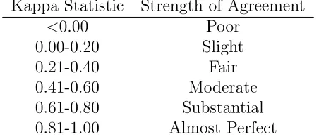
2.6.1. Cervical Cancer Diagnoses
As originally reported by Holmquist, McMahan and Williams [27], ratings for the classification of carcinoma in situ of the uterine cervix from seven pathologists were recorded. Each rater gave their interpretation of 118 slides and rated each slide as one of the following five ordinal categories: negative, atypical squamous hyperplasia, carcinoma in situ, squamous carcinoma with early stromal invasion, and invasive carcinoma. Both Landis and Koch [32] and Landis et. al. [31] investigated these data to assess rater agreement and to test for potential rater bias. These data will now be assessed to determine whether the levels of agreement within each response are equivalent and can be jointly modeled, or whether an assumption of homogeneity of ICCs for each response is violated.
2.6.2. Face Recognition
or ’psychosis spectrum’. Each subject was shown 3D images of 40 faces and asked to specify an emotion on each face from happy, sad, anger, fear or neutral. This study has the primary goal of establishing a cohort to follow to better understand the factors leading to psychosis. However, we wish to examine the level of agreement of face recognition among healthy, developed subjects. Therefore, the ratings of a subset of 73 subjects 18 or older who are typically developing with medical rating 0 will be analyzed to measure the level of agreement of facial recognition among healthy volunteers.
2.6.3. Application Results
overall ICC from the multinomial-Dirichlet distribution does not accurately portray the true level of agreement among responses due to the lack of homogeneity, and re-searchers should consider the levels of agreement among the 5 item-wise responses as an alternative. This may not be a surprising result for the cervical cancer diagnosis data, but is unexpected for the facial recognition data. One would posit that typically developing, healthy 18–21 year old subjects would be able to agree on the emotions displayed on 40 artificial faces, but clearly this is not the case. Therefore, caution should be taken when using these facial recognition results as outcomes for research as even healthy subjects do not agree what emotions are being shown.
Table 2.2: Application Results
Cervical Cancer Results Face Recognition Results Category πˆ ρˆ SE( ˆρ) Category πˆ ρˆ SE( ˆρ) Negative .281 .518 .046 Happy .207 .861 .043 Atyp. Hyperplasia .254 .147 .033 Sad .194 .573 .060 Ca in Situ .364 .377 .042 Anger .171 .660 .065 Ca w/ Early Invas. .074 .184 .054 Fear .198 .638 .062 Invasive Cancer .027 .546 .137 Neutral .230 .593 .060
Overall ICC .332 .028 .637 .031
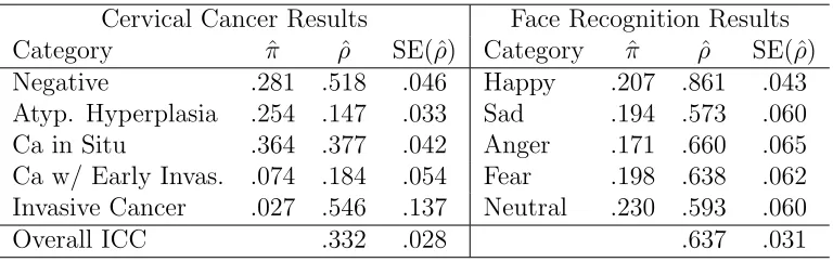
2.7. Conclusion
Figure 2.2: Application Results Distribution of -log10 P-values
Cancer Diagnosis Results
Ordered Likelihood−Ratio Test
−log10 P−v
alue
0
5
10
15
20
Face Recognition Results
Ordered Likelihood−Ratio Test
−log10 P−v
alue
0
5
10
15
20
slightly liberal, type I error rate when using Benjamini-Hochberg correction. This test is applicable to any number of potential multinomial outcomes, however simulations were completed on only the case of a four-outcome response. The test was observed to have increased power when the number of subjects, number of raters or majority
ρ· was increased. Finally, in addition to testing the homogeneity of ICCs, this test
CHAPTER 3
Estimation and Inference of the Three-Level Intraclass
Correlation Coefficient for Binomial Data
3.1. Introduction
Many different methods have been developed to assess inter-rater agreement on re-peated measures on the same object. In studying the measures of agreement and reliability of measuring a particular object multiple times, the intraclass correlation coefficient (ICC) has been proposed as a measure of agreement. Given normal, con-tinuous data, the ICC can be relatively easily calculated using the one-way random effect model yijk =µ+sij+ijk where ijk ∼N(0, σe2) andsij ∼N(0, σs2) for the kth
rating for the jth object in the ith nested-level [34]. The ICC can then be calculated
from the model asσ2s/(σs2+σe2). [21]. For the continuous case, the normality assump-tion can generally be satisfied and few issues arise in inference. Inference procedures are also straightforward given normal continuous data as presented in Searle [47].
Typically, only the object-level agreement is considered. However, this object-level agreement can be nested within other levels of agreement, artificially inflating the ob-served object-level agreement if the nested-level agreement is not taken into account. The correlation that can be found among ratings within a site, for example, can artifi-cially inflate the object-level ICC. As shown by Landis et. al. [31], the random effects model for object and nested-level effects can be written as yijk = µ+ci+sij +ijk
where ijk ∼ N(0, σ2e), sij ∼ N(0, σ2s) and ci ∼ N(0, σ2c). Then, the nested-level
ICC is calculated as σ2
c/(σc2+σs2+σ2e); whereas the object-level ICC is calculated
as (σ2
observations within a nested-level, there is currently no method to determine the corresponding standard error of the nested-level agreement.
Given dichotomous binary responses, the normality assumption is not verified and issues can arise in calculating confidence intervals and standard errors. Landis and Koch [34] showed the consistency of the point estimate of the ICC in the dichoto-mous case using the one-way random effects model, however challenging issues still arose with deriving a simplified version of the linearized Taylor-series based variance estimator for the ICC. Koch et. al. [29] developed a general method of estimation for repeated measures of categorical data that allows for asymptotic estimation of the standard error of the ICC estimate, but this method requires ≥ 5 observations per cluster to be valid and requires expressing the ICC estimator as a compounded func-tion of the underlying multinomial proporfunc-tions, leading to a series of matrix products to formulate the variance estimators. As an improvement, Mak [39] developed an ”exact asymptotic” variance of the ICC with dichotomous outcomes using the one-way random effects ANOVA model. This model provides more accurate standard errors than using methods that assume normality. However, none of these models work optimally on binary data and are not sufficient to estimate the standard error of the nested-level ICC.
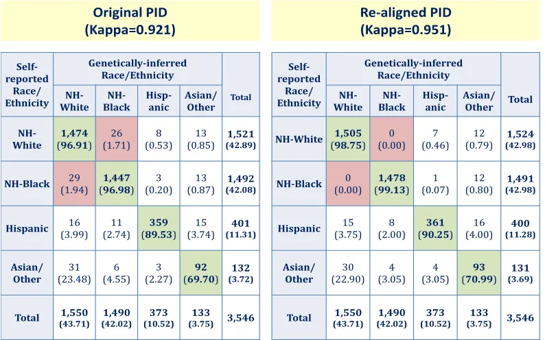
level of agreement existing among different objects within the same nested level artifi-cially inflates the estimate of the object-level agreement and will provide a nested-level adjusted object-level correlation that will better reflect the true level of agreement among objects. Finally, we will apply this method to the actual race/ethnicity classi-fication data arising from a genome-wide association study (GWAS) in which serious identity misalignment was discovered. Comparison of self-reported race/ethnicity and genetically-inferred race/ethnicity, separately within each of 47 genotyping plates, led to isolation of several genotyping plates with substantial misalignment of study sub-ject identity with mis-matched genotyping plate results.
3.2. Notation and Motivation
3.2.1. Motivating Example: Investigating Identity Misalignment within a GWAS
Table 3.1: Agreement between Self-Reported and Genetically-Inferred Ethnicity
Self-reported
Race/ Ethnicity
Genetically-inferred Race/Ethnicity
Total
NH-White Black NH- Hisp- anic Asian/ Other
NH-White (1,50598.75) (0.00) 0 (0.46) 7 (0.79) 12 (42.98) 1,524
NH-Black (0.00) 0 (1,478 99.13) (0.07) 1 (0.80) 12 (42.98) 1,491
Hispanic (3.75) 15 (2.00) 8 (90.25361) (4.00) 16 (11.28) 400
Asian/ Other
30 (22.90)
4 (3.05)
4 (3.05)
93
(70.99) (3.69) 131
Total (43.71) 1,550 (42.02) 1,490 (10.52) 373 (3.75) 133 3,546
Self-reported Race/ Ethnicity
Genetically-inferred Race/Ethnicity
Total
NH-White Black NH- Hisp- anic Asian/ Other
NH-White (1,47496.91) (1.71) 26 (0.53) 8 (0.85) 13 (42.89) 1,521
NH-Black (1.94) 29 (1,447 96.98) (0.20) 3 (0.87) 13 (42.08) 1,492
Hispanic (3.99) 16 (2.74) 11 (89.53359) (3.74) 15 (11.31) 401
Asian/ Other
31 (23.48)
6 (4.55)
3 (2.27)
92
(69.70) (3.72) 132
Total (43.71) 1,550 (42.02) 1,490 (10.52) 373 (3.75) 133 3,546 Original PID
(Kappa=0.921)
Re-aligned PID (Kappa=0.951)
Note: Cell proportions are displayed as row percentages to illustrate the accuracy of the genetically-inferred race/ethnicity within each self-reported category
increasing from 0.92 to 0.95.
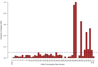
Figure 3.1: Distribution of Self-Reported Hispanics by Plate in a GWAS
CA
G−1
1 2 3 4 5 6 7 8 9 10 11 12 13 14 15 16 17 18 19 20 21 22 23 24 25 26 27 28 29 30 31 32 33 34 35 36 37 38 39 40 41 42 43 44 TP−1 TP−2 GWAS Genotyping Plate Number
Propor
tion of Hispanic PIDs
0.0 0.2 0.4 0.6 0.8 1.0
To focus particular attention on the impact of object-level clustering on ICC mea-sures of agreement, four separate category-specific binary ICCs were estimated for each race/ethnicity category in Table 3.2. The level of agreement among subjects was obtained via the 2-level variance components model, which is asymptotically equivalent to using the beta-binomial model to assess agreement [15]. The level of agreement among responses within the same genotyping plate was obtained using the methods described in Landis et. al. [31]. These methods are used to determine the subject-level agreementρand the plate-level agreementρc. As can easily be seen, the
level of agreement among subjects is very high, while the level of agreement among results within the same plate is low. However, looking at the results from Hispanic subjects, we see that the intraclass correlation coefficient for results within a plate is 0.427, which corresponds to a moderate level of agreement for responses that should be uncorrelated, according to the criteria set out by Landis and Koch [33] . How-ever, this method for assessing the ICC of responses within the same plate has a drawback. The method of deriving the standard error of the ICC estimate specified in [31] required estimating the variance/covariance matrix of the expected ANOVA mean squares estimates. This research did not provide formulas for the corresponding variance/covariance matrix, leaving a need for an explicit formula for the standard error of the nested-level ICC.
raters on the same object.
3.2.2. Notation
Understanding the roles of ”raters”, ”objects” and ”nested-levels” are crucial to un-derstanding the methods presented in this paper. In this context of rater-agreement, ”objects” will refer to the item being rated and ”raters” will refer to the process assigning the ratings. A ”nested-level” refers to a grouping that could be applied to all ”objects” such that each ”object” has an identity in one and only one ”nested-level”. For example, in the motivating GWAS example, the ”object” being rated is the race of each subject and the ”raters” refer to either the subjects’ self-assessment of race or the genetically determined race. The ”nested-level” is considered to be the genotyping plate as each subject was assigned to one and only one genotyping plate.
Letyijk be a binary outcome (0 or 1) for thekth rater (k = 1, ..., nij·) on thejth object
(j = 1, ..., ni··) in the ith nested-level (i = 1, ..., n···), and let y be the vector of all
responses. yijk is assumed to follow a binomial distribution where E(yijk) = π and
V ar(yijk) =π(1−π). Letπ be the proportion of objects with the trait being assessed
such thatP (yijk= 1) =π. Let ρ be the object-level intraclass correlation coefficient
and ζ be the nested-level intraclass correlation coefficient. Given nij· ratings per
object, the sum of all responses for an object can be written as xij = nij· P
k=1
yijk, while
the sum of all responses within a nested-level can be written as xi· =
ni·· P
j=1
nij· P
k=1
yijk. Let
xijand xi·be vectors that contain the sum of responses for all object or nested-levels
for the ith nested-level for the jth object. Let mi = ni·· P
j=1
nij· 2
!
/
ni··
P
j=1
nij·
2
, which can be interpreted as the proportion of area of the upper diagonal of the correlation matrix contributed to by the object-level ICC contributes towards. Letdi =miρ+ (1−mi)ζ,
3.3. Obtaining the Variance of
x
i·3.3.1. Estimation of the Variance of xij
In general, when multiple raters assess the same object, the results are correlated together. When studying the reliability of the raters’ assessments, that correlation is of high interest. For the typical object level ICC estimation, the correlation ρamong ratings within each object is assumed to be constant while ratings on different objects are considered to be independent. Given nij· ratings per object, the vector of all
re-sponses for an object will have annij·xnij·dimension correlation matrix in the form of
Σij·=
1 ρ . . . ρ
ρ . .. . . ... ..
. . . . 1 . . . ... ..
. . . .. ρ
ρ . . . ρ 1
(3.1)
Then a consistent estimate of the proportion π is
ˆ
π=
n··· P
i=1
ni·· P
j=1
nij· P
k=1
yijk
n··· P
i=1
ni·· P
j=1
nij·
(3.2)
As the theory is developed further, it is important that any ICC estimate allows for varying number of replicate observations per object. Restricting analysis only to objects with a certain number of ratings is unrealistic, so the theory must be kept robust to account for these cases.
response in the covariance matrix. Given the correlation matrix for multiple ratings on the same object, the variance for the total number of responses within an object can be written as
V ar(xij) = nij· X
k=1
V ar(yijk) + 2
X
p<q
Cov(yijp, yijq)
=nij·π(1−π) + 2
nij·
2
Cov(yijp, yijq)
=nij·π(1−π) +nij·(nij·−1)Cov(yijp, yijq)
=nij·π(1−π) +nij·(nij·−1)ρπ(1−π)
=nij·π(1−π) [1 + (nij·−1)ρ] (3.3)
As a result, it is clear that an over dispersion parameter exists that inflates the variance of correlated binomial data more than independent binomial data. However, the correlation due to this over dispersion increases in the presence of a nested level of correlation.
3.3.2. Estimation of the Variance of xi·
When a nested-level of correlation exists beyond object-level correlation, the correla-tion matrix of xij no longer contains all of the information regarding xi·. Therefore,
the entire xi· needs to be considered as the cluster of interest rather than the object
level xij. The correlation matrix for the vector of responses within a nested-level
contains two parameters, the object-level ICC, ρ, and the nested-level ICC, ζ. This correlation matrix can be expressed by a combination of object and nested-level cor-relations. Let 1i·· be a Pnj=1i·· nij·×Pnj=1i·· nij· matrix with all matrix elements equal
correlation matrix for nested-leveli can be written as
Σi·· =DIAG(Σi1·−ζ1i1·,Σi2·−ζ1i2·, ...,Σini···−ζ1ini···) +ζ1i·· (3.4)
Then we can find the nested-level variance in a similar fashion as the object-level variance. Recall that mi is the proportion of area of the upper diagonal of the
correlation matrix that the object-level ICC contributes towards. Then:
V ar(xi·) =
ni·· X
j=1
nij·
!
π(1−π) "
1 +
ni·· X
j=1
nij·−1
!
[miρ+ (1−mi)ζ]
#
(3.5)
The details of this derivation can be found in Appendix A.2. This variance looks similar to the variance of xij with two exceptions:
1. The number of responses for xij is the number of responses per object while the
number of responses forxi· is the number of responses within the entire cluster
2. The object-level ICC in xij is replaced by a mixture of the object and
nested-level ICCs proportional to the area of the covariance matrix occupied byρ.
This necessitates that a method should be developed such that this nested-level over dispersion parameter can be accounted for. The beta-binomial distribution will allow for the accurate modeling of the first two moments of the correlated binomial data.
3.4. Current ICC Methods
3.4.1. Object-Level ICC Estimation Framework
The beta-binomial distribution can be specified as
n k
is sum of the responses in the trial and α and β are the parameters of the model to be fit. If y ∼ Beta-binomial (α, β), then E(y) = nα/(α+β) and Var(y) = [nαβ(α+β+n)]/(α+β)2(α+β+ 1). As demonstrated earlier, E(xij)=nij·π,
which means that π=α/(α+β). It follows that 1−π=β/(α+β) as described by Crowder[16]. As a result, the variance can then be written as
V ar(xij) =
nij·π(1−π) [α+β+nij·]
α+β+ 1
=nij·π(1−π)
1 + (nij·−1)
α+β+ 1
=nij·π(1−π)
1 + (nαij·−1)
π + 1
=nij·π(1−π)
1 + π(nij·−1)
π+α
(3.6)
Recall from earlier that V ar(xij)=nij·π(1− π) [1 + (nij·−1)ρ] and π=α/(α+β).
This leads to the solution ρ=π/(π+α). Thenα=π(1−ρ)/ρ and
β = (1−π) (1−ρ)/ρ.
Now instead of optimizing the beta-binomial distribution overαandβ, the likelihood can be maximized over π and ρ. Then the log likelihood can be expressed as
LogL(π, ρ|Xij =xij) =
n··· X
i=1
ni·· X
j=1 "
log
nij· xij
+
xij−1
X
a=0
log
xij+π
1−ρ
ρ −1−a
+
nij·−xij−1
X
b=0
log
nij·−xij + (1−π)
1−ρ
ρ −1−b
− (3.7)
nij·−1 X
c=0
log
nij·+
1−ρ
ρ −1−c
#