Nucleation, Growth And Transformations In Dna Linked Colloidal Assemblies

University of Pennsylvania

ScholarlyCommons

Publicly Accessible Penn Dissertations

2016

Nucleation, Growth And Transformations In Dna

Linked Colloidal Assemblies

Ian Collins Jenkins

University of Pennsylvania, [email protected]

Follow this and additional works at:

https://repository.upenn.edu/edissertations

Part of the

Chemical Engineering Commons

This paper is posted at ScholarlyCommons.https://repository.upenn.edu/edissertations/2361

For more information, please [email protected].

Recommended Citation

Jenkins, Ian Collins, "Nucleation, Growth And Transformations In Dna Linked Colloidal Assemblies" (2016).Publicly Accessible Penn Dissertations. 2361.

Nucleation, Growth And Transformations In Dna Linked Colloidal

Assemblies

Abstract

The use of short, synthetic DNA strands to mediate self-assembly of a collection of colloidal particles into ordered structures is now quite well established experimentally. However, it is increasingly apparent that DNA-linked colloidal assemblies (DLCA) are subject to many of the processing challenges relevant to atomic materials, including kinetic barriers related to nucleation and growth, defect formation, and even diffusionless transformations between different crystal symmetries. Understanding, and ultimately controlling, these phenomena will be required to truly utilize this technology to make new materials.

Here, I describe a series of computational studies—based on a complementary suite of tools that includes Brownian dynamics, free energy calculations, vibrational mode theory, and hydrodynamic drag analysis—that address several issues related to the nucleation, growth, and stability of DNA-linked colloidal assemblies. The primary focus is on understanding the nature of the apparently enormous number of diffusionless solid-solid phase transformations that occur in crystallites assembled from DNA-functionalized colloidal particles. We find that the ubiquitous nature of these transformations is largely due to the short-ranged nature of DNA mediated interactions, which produces a panoply of zero-energy barrier pathways (or zero frequency vibrational modes) in a number of crystalline configurations. Furthermore, it is shown that hydrodynamic drag forces play a key role in biasing the transformations towards specific pathways, leading to unexpected order in the final arrangements. Additional studies also highlight how heterogeneity in the surface density of DNA strands grafted onto the particles may be used to improve nucleation and growth behavior, which is generally difficult in systems near the ‘sticky-sphere’ limit in which the interaction range is short relative to the particle size. In the final chapter of the thesis, a general and powerful technique is presented for extracting particle-particle interactions directly from particle trajectory data.

Degree Type Dissertation

Degree Name

Doctor of Philosophy (PhD)

Graduate Group

Chemical and Biomolecular Engineering

First Advisor Talid Sinno

Keywords

Colloids, DNA, Self-assembly

Subject Categories Chemical Engineering

NUCLEATION, GROWTH AND TRANSFORMATIONS IN DNA LINKED COLLOIDAL ASSEMBLIES

Ian C. Jenkins A DISSERTATION

in

Chemical and Biomolecular Engineering

Presented to the Faculties of the University of Pennsylvania in

Partial Fulfillment of the Requirements for the Degree of Doctor of Philosophy

2017

Supervisor of Dissertation

________________________

Talid Sinno, Professor of Chemical and Biomolecular Engineering

Graduate Group Chairperson

________________________

Dr. John C. Crocker, Professor of Chemical and Biomolecular Engineering

Dissertation Committee

ii

ABSTRACT

NUCLEATION, GROWTH AND TRANSFORMATIONS IN DNA LINKED COLLOIDAL ASSEMBLIES

Ian C. Jenkins Talid Sinno

The use of short, synthetic DNA strands to mediate self-assembly of a collection of colloidal particles into ordered structures is now quite well established experimentally. However, it is increasingly apparent that DNA-linked colloidal assemblies (DLCA) are subject to many of the processing challenges relevant to atomic materials, including kinetic barriers related to nucleation and growth, defect formation, and even diffusionless transformations between different crystal symmetries. Understanding, and ultimately controlling, these phenomena will be required to truly utilize this technology to make new materials.

iv TABLE OF CONTENTS

ABSTRACT

...

II

 

LIST

OF

ILLUSTRATIONS

...

VII

 

1.

INTRODUCTION

...

1

 

1.1 DNA Mediated Self-Assembly ... 1 

1.2 Numerical Simulations of DNA Functionalized Particles... 11 

1.3 Thesis Outline ... 22 

2.

A

CASE

STUDY:

PHASE

TRANSFORMATIONS

IN

CSCL

SUPERLATTICES

...

24

 

2.1 Introduction ... 24 

2.2 Langevin Dynamics Simulations ... 29 

2.3 Vibrational Mode Analysis ... 41 

2.4 Hydrodynamic Correlation and Anisotropic Diffusion ... 57 

2.5 Conclusions ... 66 

v

3.1 Introduction ... 69 

3.2 Asymmetric Interaction Matrices ... 71 

3.3 Asymmetry in Size and Interaction ... 81 

3.4 Phase Transformations Beyond the CsCl Superlattice Family ... 90 

3.5 Conclusions ... 94 

4.

THE

SUPRISING

ROLE

OF

INTERACTION

HETEROGENEITY

IN

COLLOIDAL

CRYSTALLIZATION

...

96

 

4.1 Introduction ... 96 

4.2 Method ... 97 

4.3 Results ... 102 

4.4 Conclusions ... 111 

5.

EXTRACTING

POTENTIALS

FROM

PARTICLE

TRAJECTORIES

...

113

 

5.1 Introduction ... 113 

5.2 Method ... 117 

5.3 Noiseless Dynamics ... 122 

5.4 Trajectory Noise ... 127 

vi

5.4.B. Measurement Uncertainty ... 130 

5.4.C. Error Analysis in the Context of Experiment ... 139 

5.5 Hydrodynamic Correlations ... 143 

5.6 Conclusions ... 146 

6.

CONCLUSIONS

...

148

 

6.1 A Case Study: Phase Transformations in CsCl Superlattices ... 148 

6.2 Exploring Zero-Energy Phase Transformations in Asymmetric Binary Systems ... 149 

6.3 The Surprising Role of Interaction Heterogeneity in Colloidal Crystallization ... 151 

6.4 Extracting Potentials from Particle Trajectories ... 152 

vii LIST OF ILLUSTRATIONS

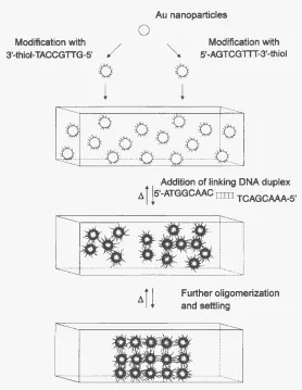
Figure 1.1. Repurposed from Ref. (26). Illustration of the process used by Mirking to assemble DNA functionalized colloidal particles. ... 4 

Figure 1.2: Repurposed from Ref. (33). Illustration of both the binary and single component systems used by Park et al which produce bcc and fcc respectively. The sticky end (colored section) of Linker A is self-complementary, while the sticky ends of Linker X and Y are only complementary with each other. ... 5 

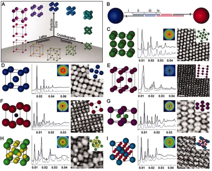
Figure 1.3: Repurposed from Ref. (35). (A) Illustration of how the three design parameters in the Macfarlane system: Lattice Parameters, Crystallographic Symmetry and Particle Size can be used to predict the structure of the lattice produced through spontaneous self-assembly. Also shown are a number of crystalline lattices which have been observed in systems of DNA functionalized nanoparticles: (C) fcc (D) bcc (E) hcp (F) CsCl (G) AlB2 (H) Cr3Si (I) Cs6C60. ... 7  Figure 1.4: Adapted from Ref. (60). Schematic representation of direct hybridization between DNA on the surface of two micron-scale particles. ... 9 

viii

strength of zero (E_AB E_AAE_BB0). A mixing ratio of 0.5 indicates both particle types

have an even mix of the two DNA types on their surface. At a mixing ratio of 0.5 all particle binding strengths are equal (E_ABE_AAE_BB). ... 10 

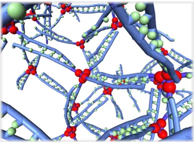
Figure 1.6: Repurposed from Ref. (63). Snapshot of a simulation utilizing the model proposed by Starr and Sciortino. The core of each functionalized particle is shown in red, single stranded DNA are shown in blue and bonding sites are shown in light green. ... 13 

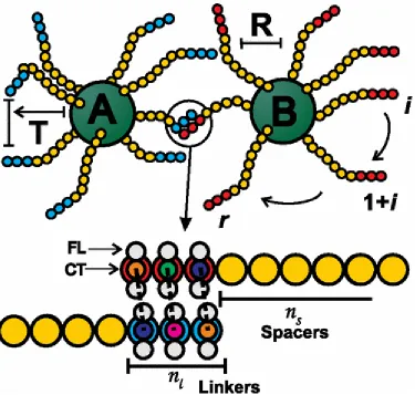
Figure 1.7: Repurposed from Ref. (65). Schematic representation of the model proposed by Knorowski, Burleigh, and Travesset. Each strand consists of ns non-bonding spacer monomers and nl bonding linker monomers. Each linker monomer is modeled with two flanker beads (FL) and a central bead (CT). ... 15 

Figure 1.8: Repurposed from Ref. (69). Schematic representation of the model proposed Leunissen and Frenkel. Each DNA strand consists of two, freely-swiveling, rigid rods. The inner rod acts as a DNA spacer and is non-interacting. The outer rod acts as the sticky, binding end to a DNA oligomer. Two different cases are shown: a) when opposing rods are tethered such that they are able to interact and b) when opposing rods are unable to interact. _i, _i and _ij are the configuration spaces accessible to rod i, rod j

and the bound i-j pair. ... 18 

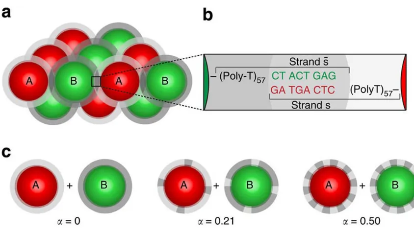
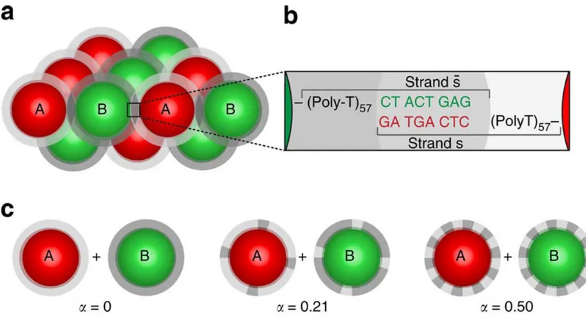
ix Figure 2.1: Adapted from Ref. (49). (A) Binary crystallite constructed from 400nm diameter particles. Interactions between particles are mediated by DNA hybridization, as shown in (B). (C) Cartoon representation of how binding strengths between unlike particle types can be controlled by modifying the density of complementary DNA on each particles surface. The α parameter is the mixing ratio, defined such that when α is 0 all DNA on the surface of type A particles is type A, and all DNA on the surface of type B particles is type B. At a mixing ratio of 0 particles of the same type have a binding strength of zero (E_AB E_AAE_BB0). A mixing ratio of 0.5 indicates both particle types

have an even mix of the two DNA types on their surface. At a mixing ratio of 0.5 all particle binding strengths are equal (E_ABE_AAE_BB). ... 25 

Figure 2.2: Adapted from Ref. (49). Sample crystallites observed in experiment. CsCl (A), CuAu-fcc (B) and fcc-SS (C) are shown. Scale bars indicate 2μm or 0.5 μm in insets. ... 27 

Figure 2.3: Adapted from Ref. (49). Two examples of DNA functionalized colloidal particle crystallites exhibiting the CsCl and CuAu superlattices simultaneously. Scale bars indicate a length of 2μm. ... 28 

Figure 2.4: Example initial system configuration for a 1500 particle seed. Non-crystal particles are shown at 10% actual size for visualization purposes... 31 

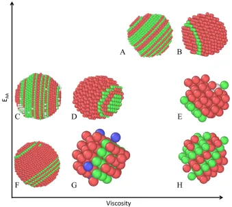
x Figure 2.6: Sample crystallites for like particle interaction strength (EAA) versus system viscosity. System parameters are (all energies in units of kBT): A)EAB 6, EAA 2.5,

0.01 _w







, n5000; B)E_AB 6, EAA 2.5,



0.05



w, n5000; C)EAB 6, 1.5

AA

E  ,





0

, n8000; D)E_AB 5, E_AA 1.5,



0.005



_w, n1500; E)E_AB 4

, E_AA 1.5,



0.05



_w, n220; F)E_AB 4, E_AA1,





0

, n8000; G)E_AB 6,

1 AA

E  ,



0.005



w, n220; H)EAB 5, EAA1,



0.05



w, n220. ... 35  Figure 2.7: Sample crystallites for crystallite size versus unlike particle interaction strength. System parameters are (all energies in units of kBT): A) EAB 4, EAA1,

0





, n8000; B) E_AB 6, E_AA2.5,





0

, n8000; C) E_AB 5, E_AA1.5,

0.005 _w







, n5000; D) E_AB 6, E_AA 1.5,





0

,n5000; E) E_AB 5,

1.5 AA

E  ,



0.005



w,n1500; F) EAB 6, EAA1.5,



0.005



w, n1500; G) 4

AB

E  , E_AA 1.5,



0.05



_w, n220; H) E_AB 5, E_AA 2.5,





0

,n220; I)

6 AB

E  , E_AA 1.5,



0.05



_w, n220. ... 36 

Figure 2.8: Sample crystallites for crystallite size versus viscosity. System parameters are (all energies in units of kBT): A) EAB 4, EAA1,





0

,n8000; B) EAB 6,

1.5 AA

E  ,



0.01



w, n8000; C) EAB 6, EAA 1.5,





0

,n5000; D) EAB 6, 1.5

AA

E  ,



0.005



_w, n5000; E) E_AB 6, E_AA2.5,



0.01



_w,n5000; F)

5 AB

E  , E_AA1.5,



0.005



_w,n1500; G) E_AB 6, E_AA 2.5,



0.05



_w,

1500

n ; H) E_AB 5, EAA 2.5,





0

,n220; I) EAB 6, EAA1,



0.005



w, 220

xi Figure 2.9: Sample crystallites for unlike particle interaction strength versus like particle interaction strength. System parameters are (all energies in units of kBT): A) EAB 6,

1 AA

E  ,



0.005



w, n220; B) EAB 6, EAA1.5,



0.005



w, n1500; C) 6

AB

E  , E_AA2.5,





0

, n8000; D) E_AB 5, E_AA 1.5,



0.005



_w, n1500;

E) E_AB 5, E_AA 2.5,





0

, n220; F) E_AB 4, E_AA1,





0

, n8000 n220

; G) E_AB 4, EAA2.5,





0

, n220. ... 38  Figure 2.10: fcc-to-hcp order parameter,



, as a function of each of the 4 simulation parameters: Unlike particle type binding strength E_AB, like particle interaction strength

AA

E fluid viscosity relative to water

 

/ _w and crystallite size N . ... 40 

Figure 2.11: Vibrational density-of-states for spherical crystallites. Frequencies correspond to the square-root of the Hessian eigenvalues. Blue – 1000-particle CuAu-I crystallite



E

_AA



E

_AB



6

k T

_B



; red – 1000-particle CsCl crystallite



E

_AB



6

k T E

_B

,

_AA



0



. ... 43 

Figure 2.12: (A) (100) plan view of an arbitrary zero-frequency eigenvector for the ideal CsCl configuration of a cubic crystallite with 200 particles. (B) (100) plan view of the center-plane “modelet” eigenvector showing center-plane particles moving along the (110) direction while all other particles are stationary. ... 45 

Figure 2.13: (100) plan views of different transformation modes constructed using linear combinations of modelets. (A) Shear, (B) “zig-zag”, and (C) Bain. ... 51 

xii the original CsCl lattice. B and E show the (100) and (010) views of the partially transformed system, after the zero frequency evolution process has been completed. C and F show the (100) and (010) views of the system once the energy minimization has terminated. ... 53 

Figure 2.15: Compositionally ordered CuAu-I (A), hcp (B) and rhcp (C) superlattice structures. Each cp structure exhibits 8 like contacts and 4 unlike contacts for every particle. ... 55 

Figure 2.16: (A) Scaled mobility of zero-frequency eigenmodes as a function of spherical CsCl crystallite size for shear – green, Bain – blue, and zig-zag – red. Scaled mobilities are reported relative to mobilities for isolated particles (see eq. 2.7). Inset: Distribution of scaled mobilities for 100 randomly selected zero-frequency eigenvectors for the 54-particle crystallite. (B) Scaled mobilities for 432-54-particle crystallite as a function of particle size relative to separation,

d

_r



(

d

_p

/ )

d

_c 1, for: shear – green, Bain – blue, zig-zag – red. ... 62 

Figure 2.17: Scaled mobilities of zero-frequency eigenmodes for 432-particle CsCl crystallite as a function of particle size relative to separation (d_r) for shear (green), Bain

(blue), and zig-zag (red) modes: Squares – rotation-free, circles – torque-free. ... 64 

xiii

Figure 3.2: Example of the pcp structure observed in LD simulation. This structure was produced by performing an LD simulation on a CsCl crystallite seed containing 1837 particles. Binding strengths between A particles (shown in red) were set to 0kBT, between B particles were (shown in green) set to 1kBT and between particles of unlike type were set to 6kBT. The CsCl crystallite rapidly transformed into the structure shown. ... 73 

Figure 3.3: Overview of the CsCl to pcp and pcp to RHCP transformations observed in LD simulations. The initial configuration, shown on the left, is a CsCl crystallite containing 1837 particles. Performing an LD simulation with this CsCl crystallite as the seed structure, with binding strengths between A particles (shown in red) set to 0kBT, between B particles (shown in green) set to 1kBT and between particles of unlike type set to 6kBT, results in rapid transformation into the pcp crystallite shown in the center. Upon increasing binding strengths between A particles to 1kBT, the crystallite transforms a second time, producing the rhcp crystallite shown on the right. ... 74 

Figure 3.4: (001) view of the pcp producing transformation. The initial transformation pathway is shown on the left, superimposed on a CsCl crystallite. The resulting pcp crystallite is shown on the right. The pcp lattice was produced by evolving a CsCl crystallite seed containing 200 particles each with a diameter of 400nm along the pcp transformation pathway using the method described in Section 2.3. A particles are shown in red, B particles are shown in green... 76 

xiv 200 particles with a diameter of 400nm along the “psuedo-shear” and “psuedo-zig-zag” transformation pathways using the zero-frequency mode evolution method described in Section 2.3. A particles are shown in green, B particles are shown in red. ... 78 

Figure 3.6: Complete diagram illustrating the transformations available to the CsCl superlattice. A particles are colored red, B particles are colored green. Bonds connecting neighboring particles indicate only that they are within interaction range of one another. The CsCl lattice is shown from its (100) orientation, and all other lattices show the same face after it has been transformed. The dotted line directly connecting CsCl to hcp indicates that while the transformation is physically possible, it is not experimentally observed due to a negative hydrodynamic bias.  ... .80 

Figure 3.7: Overview of the CsCl to RIrV transformation process observed in LD simulations. The initial configuration, shown on the left is a CsCl crystallite containing 4285 particles. Performing an LD simulation with this CsCl superlattice as the seed structure, with binding strengths between A particles (shown in red) set to 0kBT, between B particles (shown in green) set to 1kBT and between particles of unlike type set to 6kBT, results in a RIrV crystallite, shown on the left. The RIrV lattice is a random combination of the HIrV and BIrV lattices. ... 82 

xv method described in Section 2.3. The 500nm type B particles are shown as green and the 425nm type A particles are shown as red. ... 84 

Figure 3.9: Overview of the Bain transformation pathway between the CsCl superlattice and the CuAu-fcc superlattice at a size ratio 0.85. Arrows indicate the displacement direction at the start of the transformation. The initial CsCl crystallite is shown on the left, and the fully transformed CuAu-fcc crystallite is shown on the right. The transformation pathway was generated and followed using the method described in Section 2.3. 500nm B particles are shown as green and 425nm A particles are shown as red... 86 

Figure 3.10: Overview of the CsCl to HIrV transformation using the pcp phase as an intermediate. Arrows indicate the displacement direction at the start of the transformation. The transformation proceeds clockwise starting from the initial CsCl crystallite shown in the upper left. The second crystallite has a pcp structure, the third structure is an intermediate between CsCl and HIrV and the fourth structure is HIrV. The 500nm B particles are shown as green and the 425nm A particles are shown as red. ... 87 

Figure 3.11: Complete diagram illustrating the transformations available to the CsCl superlattice at a size ratio of 0.85. A particles are colored red, B particles are colored green. Bonds connecting neighboring particles indicate are within interaction range. The CsCl lattice is shown from its (100) orientation, and all other lattices show the same face after it has been transformed. The dotted line directly connecting CsCl to HIrV indicates that while the transformation is physically possible, it is not experimentally observed due to hydrodynamic biases. ... 89 

xvi and 0.565, respectively. In the range between 0.565 and 0.73, no crystallites have been observed experimentally. ... 90 

Figure 3.13: Example of a single (100) NaCl superlattice modelet. Only a single column of particles in the (100) direction are associated with this modelet. Particles are shown at a size ratio of 0.565. Type A particles are colored red and have a radius of 158nm, type B particles are colored green and have a radius of 280nm. ... 91 

Figure 3.14: (-110) (A) and (001) (B) perspective of the (110) shear in the NaCl superlattice. The initial transformation pathway is shown on the left, the final product structure is shown on the right. A crystallite containing 110 particles at a size ratio of 0.565 was used. A particles are colored red and have a radius of 158nm, B particles are colored green and have a radius of 280nm. ... 93 

Figure 4.1: Interaction heterogeneity reduces nucleation barrier height and critical nucleus size, particularly at weaker average binding. (a) Barrier height as a function of heterogeneity: purple –



U 3.0, blue –



U 3.2, green –



U 3.4, orange –

3.8

U



 , red –



U 4.0. (b) Free energy profiles as a function of cluster size for

3.2

U



 : blue –

p



0

, green –

p



0.05

, red –

p



0.10

. ... 104 

Figure 4.2: Radial fractionation of binding strengths in clusters: blue –



U 3.0,

0.39

p



, red –



U 3.4,

p



0.25

, and black –



U 5.5,

p



0.05

. Insets: mid-plane slices through crystallites showing binding strength distribution; green is the mean value (b = 1), yellow/red is higher, cyan/blue is lower. ... 106 

xvii window. (a) Evolution of the crystallite count for different combinations of average binding strength and population heterogeneity: black diamonds –



U 5,

p



0

; blue circles –



U 4.8,

p



0.05

; green squares –



U 5.4,

p



0

. (b-g) Final configurations as a function of interaction strength for p = 0 [top row,



U  4.8 (b), 5.2

(c), and 5.8 (d)] and p = 0.15 [bottom row,



U  3.6 (e), 4.0 (f), and 4.6 (g)]. Particle

color represents binding strength: green is the mean value, red is higher, blue is lower. ... 108 

Figure 4.4: Interaction heterogeneity lowers and widens the window for crystallization. Color field denotes the maximum cluster number density, , as a function of average binding strength and heterogeneity. Thin lines represent isolines of nucleation barrier height,





G

_max, with values (upper left to lower right): 1, 2, 3, 5, 30, and 90 kBT. Dashed lines schematically denote crystallization window. Diamond symbols show locations of corresponding to the configurations snapshots shown in Figure 4.3. ... 110 

Figure 5.1: Pair interaction potentials (blue lines and squares) and force profiles (red lines and circles) extracted from observing a system of 64 Lennard-Jones particles evolving via (a) inertial dynamics and (b) overdamped dynamics. Extracted profiles, which are generated using 60 0.075



-width square wave basis functions, are shown by symbols; input profiles are denoted by the solid lines. 500 force evaluations were used to construct the profiles in each case. ... 123 

Figure 5.2: Error as a function of total trajectory data points for a system of 64 Lennard-Jones particles evolving via inertial dynamics. Error is calculated as *

2 M



F F ,

xviii function,

F

is the actual force at each of these points, and M is the number of comparison points (bins). Error is computed over the range

1.2



 

r

4.5



, which is sampled by all trajectories. Four square wave discretization levels were considered: 60 basis functions (red squares), 20 basis functions (orange circles), 10 basis functions (green diamonds) and 5 basis functions (blue triangles) over the interval

0

 

r

4.5



. Also shown is the error for the 60 line-segment basis function set (gold crosses). ... 126 

Figure 5.3: Potential function (blue line and squares) and force profile (red line and circles) extracted from a system of 64 Lennard-Jones particles evolving via Brownian dynamics. Extracted profiles, which are generated using 60 0.075



-wide square wave basis functions, are shown by symbols; input profiles are denoted by solid lines. 500 force evaluations were used to construct the profiles. Inset: Error difference in the force profiles extracted from overdamped (fluctuation free) and Brownian dynamics trajectories. ... 129 

Figure 5.4: Force profiles extracted from inertial trajectories free of thermal fluctuations but subject to measurement uncertainty using 500 (left column) or 10000 (right column) force evaluations. Measurement uncertainty magnitude is 0.03 (top row), 0.3 (middle row), and 1.5 (lower row) of the mean particle displacement between two successive observations. In each panel, the input force profile is shown as a solid red line. The dashed blue line represents the best-fit LJ force profile using a single scalar multiplier. All extracted profiles are generated using 60 square wave basis functions of width 0.075



. ... 132 

xix Figure 5.6: Force profiles extracted from observing a system of 64 Lennard-Jones particles evolving via inertial dynamics subject to measurement uncertainty of amplitude 0.525. Extracted profiles are shown by symbols (uncorrected force – circles, corrected force – diamonds), the input force profile is denoted by the solid red line. The dashed blue line shows the best-fit LJ force profile for the uncorrected force assuming that the input force is scaled by a single multiplier of 1.58. Both extracted profiles are generated using a set of 60 square wave basis functions of width 0.075



. ... 136 

Figure 5.7: Difference in the force profile error extracted from noisy and exact inertial dynamics trajectories as a function of the force evaluation count calculated for several measurement uncertainty amplitudes (relative to average particle displacement): orange circles –described in the text (which has been corrected for using eq. (5.18)). ... 138 

Figure 5.8: Error as a function of time step size for a system of 64 Lennard-Jones particles evolving via exact, noiseless, inertial dynamics. Extracted force profiles, are generated using 60 0.075



-wide line segment basis functions. Error is calculated as

*

2 M



F F , where _F* _{contains the force calculated from eq. (5.13) at the midpoint}

of each basis function,

F

is the actual force at each of these points, and M is the number of comparison points (bins). ... 142 

1

1. INTRODUCTION

1.1 DNA Mediated Self-Assembly

Equation Section 1

Self-assembly is any process in which a system of distinct components spontaneously self-organizes into a larger, more complex, ordered structure. Self-assembly is found throughout nature, from ice crystals forming in water to the growth of nearly every living organism. The complexity of structures produced through such self-assembly processes greatly surpasses what can be designed and built manually. In order to match the level of complexity present in nature we must learn to use its primary tool, self-assembly.

The science of self-assembly has undergone significant development since its inception. A variety of approaches for producing component parts capable of both spontaneous and induced assembly have been developed, varying both with regard to the underlying mechanisms responsible for driving the assembly processes, such as electrostatics (1-3), magnetics (4-6), depletion effects (7), and even fluid flow (8), and the length-scale of the component particles, which range from the nano through the micro scale (9) and beyond (10). Through both experiment and simulation it has been demonstrated that human-designed self-assembling systems are capable of producing an enormous variety of structures and a significant amount of research has been done to optimize these systems both in regard to the robustness of the growth process and the accuracy of the final product structure (11-14).

2 strands of DNA with complementary nucleotide sequences come into contact. Once in contact each individual complementary nucleotide base pair forms a hydrogen bond, linking the strands together. The hybridization of single-stranded DNA has been employed in a variety of ways to induce self-assembly behavior in in systems comprised purely of DNA as well as in systems in which other objects are guided by DNA. In the former case a wide variety of structures have been assembled, including nanotubes(15, 16), 2D crystals(17), 3D periodic arrays(18) as well as a variety of structures built from DNA bricks(19, 20) and origami(21-25). However, there are two significant drawbacks to using DNA in this manner. First, by relying entirely upon DNA as a construction material, you are limited to producing structures which exhibit the thermal, electrical and optical properties of DNA. Second, and more importantly, DNA is costly to produce, making large scale production of materials constructed entirely of DNA prohibitively expensive. It is possible to simultaneously avoid both of these issues by using a second, less expensive material, such as polystyrene, as the bulk material, while still relying on DNA to drive the self-assembly process. This second approach is the focus of my research.

4 Figure 1.1. Repurposed from Ref. (26). Illustration of the process used by Mirking to assemble DNA functionalized colloidal particles.

5 particles, in turn allowing the self-assembly process to occur at much higher temperatures. At these higher temperatures DNA hybridization is reversible allowing the hybridized DNA to dynamically dissociate and reform. With the particles able to dynamically connect and disconnect, the growth of ordered crystallites becomes possible. Initially only two ordered crystal lattices were observed. The first, with face centered cubic (fcc) symmetry, occurred when only one species of single-stranded DNA was used to functionalize particles. In such a system, the freely floating duplexes are symmetric and interaction between all particles is identical. The second lattice, with body centered cubic (bcc) symmetry, was only observed in multi-component systems. Here, two particle-bound DNA species were employed, and each particle was functionalized with only a single type of DNA oligomer. In this particular binary system, the DNA sequences were chosen such that only particle pairs functionalized with different species of DNA were able to bond. The system used by Park et al is illustrated below in Figure 1.2.

7 Figure 1.3: Repurposed from Ref. (35). (A) Illustration of how the three design parameters in the Macfarlane system: Lattice Parameters, Crystallographic Symmetry and Particle Size can be used to predict the structure of the lattice produced through spontaneous self-assembly. Also shown are a number of crystalline lattices which have been observed in systems of DNA functionalized nanoparticles: (C) fcc (D) bcc (E) hcp (F) CsCl (G) AlB2 (H) Cr3Si (I) Cs6C60.

8 interaction range ratio at these particle size scales makes ordered structures more difficult to grow, typically resulting in lower quality crystallites than are observed at the nanoscale. In large part this relative difficulty arises because micron-scale particles are closer to the ‘sticky-sphere’ limit (57) where entropic barriers act to slow down and inhibit assembly. On the other hand, micron-scale particles are of great interest for assembling ordered metamaterials (58) with interesting photonic and/or phononic properties. Although this goal has not yet been achieved, significant progress has been made in improving the crystallization behavior at this length-scale and identifying what crystal lattices are achievable. The work in this thesis is aimed precisely at elucidating the various mechanisms by which micron-scale particle assemblies nucleation, grow and transform.

9 Figure 1.4: Adapted from Ref. (60). Schematic representation of direct hybridization between DNA on the surface of two micron-scale particles.

10 Figure 1.5: Adapted from Ref. (49). (A) Binary crystallite constructed from 400nm diameter particles. Interactions between particles are mediated by DNA hybridization, as shown in (B). (C) Cartoon representation of how binding strengths between unlike particle types can be controlled by modifying the density of complementary DNA on each particles surface. The α parameter is the mixing ratio, defined such that when α is 0 all DNA on the surface of type A particles is type A, and all DNA on the surface of type B particles is type B. At a mixing ratio of 0 particles of the same type have a binding strength of zero (E_AB E_AAE_BB0). A mixing ratio of 0.5 indicates both particle types

11

1.2 Numerical Simulations of DNA Functionalized Particles

Precisely and accurately constructing DNA functionalized particles at both the nano- and micro-scales is very challenging. Simulations offer a means to study these systems while avoiding this rather difficult assembly process. However, direct, explicit simulation of the various components of a system of DNA functionalized particles can be very computationally demanding. In order to successfully simulate such a system on a useful timescale, it is necessary to use a coarse grained model for the interactions between particles.

One common approach is to simulate the DNA oligomers using a method based on bead-spring polymer models (61, 62). One of the first examples of this approach is the model developed by Starr and Sciortino (63) which was designed to simulate the system studied by Stewart and McLaughlin (64). In this nanoscale system the DNA duplexes often used to mediate interactions between DNA functionalized particles are excluded. Instead, the single-stranded DNA sequences are chosen such that they are directly complementary. Additionally, each particle in this system is functionalized with only four strands of DNA in a tetragonal configuration. In the model each pair of neighboring monomers in a DNA strand are connected through a finitely-extensible, non-linear elastic anharmonic spring potential of the form

2 2

0

0

( ) ln 1

2 FENE kR r U r R  _{ }      _{  }  _{ }   

. (1.1)

12

 



1 cos



l

U

_



k





, (1.2)

13 Figure 1.6: Repurposed from Ref. (63). Snapshot of a simulation utilizing the model proposed by Starr and Sciortino. The core of each functionalized particle is shown in red, single stranded DNA are shown in blue and bonding sites are shown in light green.

15 Figure 1.7: Repurposed from Ref. (65). Schematic representation of the model proposed by Knorowski, Burleigh, and Travesset. Each strand consists of ns non-bonding spacer monomers and nl bonding linker monomers. Each linker monomer is modeled with two flanker beads (FL) and a central bead (CT).

16 of more implicit, coarse grained models (65-79). One such model is used by Largo et al.

(80) and Theodorakis et al. (81) in which Metropolis Monte Carlo (MMC) simulations of two DNA functionalized nanoparticles, simulated using the previously described approach developed by Starr and Sciortino (63), are used to generate statistical information about the relative orientation and center-to-center distance of pairs of particles. These statistics are then used to determine the probability of finding the system in any given configuration, where the configuration is assumed to be entirely described by the orientations of the two particles, (₁,₂) and their center-to-center distance. Here, _i is defined as the smallest angle between any DNA strand on particle

i

and the center-center vector between particles. This probability distribution,



, ,

1 2



p r

 

, is then used to calculate the effective potential between the two particles using the expression



















1 2



1 2

1 2

ln

, ,

, ,

ln

, ,

p r

U r

p r

 

 

 





, (1.3)

where r is any distance beyond the maximum interaction range of the particles.

17 is allowed to freely swivel about its connection to the inner rod and interacts with other outer rods according a two state potential: bound or unbound, such that there is a constant energy associated with binding. A schematic representation of this system is shown in Figure 1.8. Once two plates have been populated with these rods they are placed a fixed distance apart and Monte Carlo moves are proposed for the rods. These moves are made by first randomly selecting a rod, i, from one of the two plates. The list of all rods, k, on the opposing plate which are within range of rod i is then generated. Next the probability of rod i binding to any particular rod, j, is calculated as

1

ij ik G ij G k

e

p

e

   







(1.4)

and the probability of forming no bond is

,

1

1 ik

i unbound G

k

p

e







, (1.5)

where G_ijis the free energy associated with the hybridization between rod i and rod j. The value of G_ijis calculated using the expression

,

0

1

ln

ij ij ij solution B

j i

G

G

k T











 





_



_

 





, (1.6)

where _i, _j and _ij are measures of the configuration space accessible to rod i, rod j

18 distances. The DNA interaction free energy as a function of separation distance can then be found using the expression

, ,

0 ,

, ,

,

( )

2

ln

ik solution ik solution

n confined

B bonds _{G h} ik solution

N n unconfined G

G h

k T

n

_

d G









 



_



_















, (1.7)

where

, ,

ik solution

bonds G h

n

_ is the number of pairs of hybridized DNA strands averaged over a specific value of G_{ik solution,} and plate separation distance.

19 unable to interact. _i, _i and _ij are the configuration spaces accessible to rod i, rod j

and the bound i-j pair.

The coarse grained model I employ for all simulations reported in this thesis was developed and confirmed against experimental data by Rogers et al.(82). This coarse grained approach begins by proposing a model for describing two micron-scale DNA functionalized colloidal particles, separated by some fixed distance, h. While the most general calculation of the interaction potential between DNA-linked particles must include terms correcting for DNA polymer non-ideality and other terms in the partition function, (69, 70, 83), for the particular DNA configuration we use, an idealized model gives an acceptably accurate result (84, 85). Additionally, while smaller particles, whose interactions may be non-pairwise additive, require explicit polymer simulations to compute the effective interaction potential(86-88), the micron-scale spheres in this study, are large enough that their interactions are demonstrably pair-wise additive and implicit polymer models can be used.

20 binning process can be used to approximate the continuous number density of DNA in the region between the two particles. A schematic representation of this process is shown below in Figure 1.9. During this process it is necessary to record two other numbers: the number of proposed strands which do not intersect the anchor sphere,

 

h





and the number of these strands which do not intersect with the opposing

sphere,



 

h

. Due to the reversible nature of DNA bridge formation, it is assumed that the equilibrium concentration of DNA bridges between two particles can be calculated using the chemical equilibrium expression

/

0 ( ) ( )

( ) A B Ghyb k TB

AB

C C

C e

C



 r r

r

, (1.8)

along with the conservation equations

0_{( ) ( ) ( )}

A A AB

C r C r C r

(1.9)

and

0_{( ) ( ) ( )}

B B AB

C r C r C r , (1.10)

where G_hyb is the hybridization Gibbs free energy, C_AB( )r , C_A( )r and C_B( )r are the equilibrium concentrations of hybridized DNA, non-hybridized DNA from particle A and non-hybridized DNA from particle B, respectively, 0_{( )}

A

C r and C_B0( )r are the values of

( ) A

21 number of DNA bridges,

N

_bridge to the attraction interaction energy between the particles is invoked (90-92)

a

bridge B

E

N k T



 

. (1.11)

The value of

N

_bridge , and therefore E_a can be calculated by integrating over the spatial bins using the expression

 

3

bridge Av AB

N

 

N



d C

r

r

, (1.12)

where N_Avis Avagadro’s number. Finally, the energy associated with entropic repulsion due to brush compression (90) can be calculated using the expression

 

 

 

ln

r

B

E h

h

k T

_

h









  

_



_







. (1.13)

22 Figure 1.9: Repurposed from Ref. (82). Schematic representation of the method used to calculate the average number density of DNA. Left: A random walk is used to propose the configuration of a DNA brush. Center: Multiple random walks with uniformly distributed tethering points. Right: The final, averaged, DNA density profile, only the final coordinate in the random walk is used in the averaging process.

1.3 Thesis Outline

24

2. A CASE STUDY: PHASE TRANSFORMATIONS IN CsCl

SUPERLATTICES

2.1 Introduction

Equation Section 2

This study was inspired by a spontaneous bcc-to-fcc diffusionless (solid-solid) transformation experimentally observed by Casey et al. (49) in DNA-assembled, micron-scale, binary colloidal superlattice crystals. Although such transformations are well-studied in atomic materials because of their considerable technological importance (e.g., Martensitic transformation in steel hardening (97) and shape memory alloys (98)), their analysis in DLPAs is essentially non-existent. Understanding the nature of such transitions in colloidal assemblies may provide additional pathways for manipulating DLPAs to produce desired configurations that are otherwise difficult or impossible to access by direct nucleation.

25 Figure 2.1: Adapted from Ref. (49). (A) Binary crystallite constructed from 400nm diameter particles. Interactions between particles are mediated by DNA hybridization, as shown in (B). (C) Cartoon representation of how binding strengths between unlike particle types can be controlled by modifying the density of complementary DNA on each particles surface. The α parameter is the mixing ratio, defined such that when α is 0 all DNA on the surface of type A particles is type A, and all DNA on the surface of type B particles is type B. At a mixing ratio of 0 particles of the same type have a binding strength of zero (E_AB E_AAE_BB0). A mixing ratio of 0.5 indicates both particle types

have an even mix of the two DNA types on their surface. At a mixing ratio of 0.5 all particle binding strengths are equal (E_ABE_AAE_BB).

28 The action of a displacive (or diffusionless), transformation was deduced based on two principal observations. First, a small number of the crystallites were found to exhibit two distinct domains (CsCl and CuAu-I) separated by a sharp, coherent interface, similar to the Martensite-Austenite interfaces observed in steels (101) as shown below in Figure 2.3. A more indirect suggestion for the presence of a diffusionless transformation between CsCl and CuAu-I came from the observation that the vast majority of CuAu-I crystallites found in experiment were perfectly ordered, in contrast to previous modeling studies performed by Scarlett et al. (99) which indicate homogeneous nucleation and growth of close-packed phases in this system give rise to numerous compositional ordering defects.

29 In the following, we first employ direct Langevin dynamics (LD) simulations and establish the feasibility of the transformation, although we find that the resulting close-packed configurations are always more structurally diverse than the uniform CuAu-I observed in experiment. We understand the source of this diversity by performing a vibrational mode analysis which enables us to identify all possible energetically degenerate transformation pathways that lead to different final (close-packed) configurations. Finally, we consider the role of hydrodynamic correlations on the effective multi-particle diffusivity of the system configuration along different transformation pathways, and find that the anomalous configurations seen in experiment are precisely those that are strongly favored by hydrodynamics. Furthermore, we conjecture that such hydrodynamic selection may play a role in other colloidal systems displaying collective particle dynamics, such as hard-sphere and attractive glasses.

2.2 Langevin Dynamics Simulations

We first performed LD simulations that consist of numerical integration of the Langevin equation for a system of particles that are subject to interparticle forces as well as forces due to the presence of an implicit solvent, i.e.,

( ) 2 _B ( )

mr F r 



r



mk TR t

(2.1)

30 so that

R

( )

t



0

and

R R

( ) ( )

t

t







(

t t





)

. All LD simulations were performed using the LAMMPS software package (102), with particle interactions calculated using the coarse-grained inter-particle pair potential model developed by Rogers et al. (82) which is described in detail in Section 1.2.

The LD simulations of CsClCuAu-I transformation were initialized by placing spherical CsCl crystallites in a colloidal fluid of randomly-placed particles corresponding to a particle volume fraction of 0.3. An example of the initial system configuration is shown below in Figure 2.4. The colloidal fluid particles were used to stabilize the crystallite against dissolution. In each run, the simulation was first allowed to reach equilibrium using interparticle interactions that favored the CsCl phase



E

_AB



6.0

k T E

_B

,

_AA



0



once equilibrium was reached the interactions were adjusted to

31 Figure 2.4: Example initial system configuration for a 1500 particle seed. Non-crystal particles are shown at 10% actual size for visualization purposes.

33

Figure 2.5: Examples of transformed crystallite configurations observed in LD simulations (see text). Crystallites initially contain 5000

(case A) or 8000 (cases B and C) particles, which are colored according to their structure as determined by CNA. Red particles are

34

In order to better quantify the differences between the rhcp structures produced by Langevin simulations of the bcc-cp transformations and those seen in experiment, an order parameter,



, was defined as the ratio of close-packed planes in the crystallite which possess fcc structure to those that possess hcp structure. A χ value of 1 would then indicate an equal distribution of fcc- and hcp-like crystallite planes. A total of 4 parameters were investigated: the crystallite size (220-8000 particles), the implicit fluid viscosity (0-500% of water), unlike interaction strength

(4

k T

_B



E

_AB



6

k T

_B

)

, and like

interaction strength

(1.0

k T

_B



E

_AA



2.5

k T

_B

)

. The range of viscosity was sufficient to span the transition from overdamped to inertial dynamics. A system of interacting particles in a viscous medium is considered overdamped when (103)

1

2

mk



_

(2.2)

where m is the particle mass, k is the effective spring constant experienced by a particle in the system and



is the drag coefficient. The drag coefficient is given by

3

d

_p







(2.3)

where μ is the fluid medium viscosity and

d

_p is the particle diameter. In the present calculations, the value of gamma for a system at 5% the viscosity of water,



_w, with 400nm-diameter particles is 3.36x10-9 _{kg/s. Furthermore, the value of}

mk when the

35 representative samples of transformed crystallites obtained at various combinations of the above parameters

Figure 2.6: Sample crystallites for like particle interaction strength (EAA) versus system viscosity. System parameters are (all energies in units of kBT): A)EAB 6, EAA 2.5,

0.01 _w







, n5000; B)E_AB 6, E_AA 2.5,



0.05



_w, n5000; C)E_AB 6,

1.5 AA

E  ,





0

, n8000; D)E_AB 5, E_AA 1.5,



0.005



_w, n1500; E)E_AB 4

, E_AA 1.5,



0.05



w, n220; F)EAB 4, EAA1,





0

, n8000; G)EAB 6, 1

AA

36 Figure 2.7: Sample crystallites for crystallite size versus unlike particle interaction strength. System parameters are (all energies in units of kBT): A) EAB 4, EAA1,

0





, n8000; B) E_AB 6, E_AA2.5,





0

, n8000; C) E_AB 5, E_AA1.5,

0.005 _w







, n5000; D) E_AB 6, E_AA 1.5,





0

,n5000; E) E_AB 5,

1.5 AA

E  ,



0.005



w,n1500; F) EAB 6, EAA1.5,



0.005



w, n1500; G) 4

AB

E  , EAA 1.5,



0.05



w, n220; H) EAB 5, EAA2.5,





0

,n220; I) 6

AB

37 Figure 2.8: Sample crystallites for crystallite size versus viscosity. System parameters are (all energies in units of kBT): A) EAB 4, EAA1,





0

,n8000; B) EAB 6,

1.5 AA

E  ,



0.01



w, n8000; C) EAB 6, EAA 1.5,





0

,n5000; D) EAB 6, 1.5

AA

E  ,



0.005



w, n5000; E) EAB 6, EAA2.5,



0.01



w,n5000; F) 5

AB

E  , E_AA1.5,



0.005



_w,n1500; G) E_AB 6, E_AA 2.5,



0.05



_w,

1500

n ; H) E_AB 5, E_AA 2.5,





0

,n220; I) E_AB 6, E_AA1,



0.005



_w,

220

38 Figure 2.9: Sample crystallites for unlike particle interaction strength versus like particle interaction strength. System parameters are (all energies in units of kBT): A) EAB 6,

1 AA

E  ,



0.005



_w, n220; B) E_AB 6, E_AA1.5,



0.005



_w, n1500; C)

6 AB

E  , EAA2.5,





0

, n8000; D) EAB 5, EAA 1.5,



0.005



w, n1500; E) E_AB 5, E_AA 2.5,





0

, n220; F) E_AB 4, E_AA1,





0

, n8000 n220

40 Figure 2.10: fcc-to-hcp order parameter,



, as a function of each of the 4 simulation parameters: Unlike particle type binding strength E_AB, like particle interaction strength

AA

41

2.3 Vibrational Mode Analysis

The persistent discrepancy between simulated and experimental transformed crystallites suggests the presence of multiple accessible transformation pathways. In this section we seek to generate a basis for identifying all possible pathways and thus a mechanism that would explain the discrepancy. We first performed a vibrational mode analysis of the CsCl (and CuAu-I) superlattice DLPAs. Note that the experimental system is overdamped and the vibrational frequencies we describe below do not imply oscillatory behavior (104). Vibrational mode analysis was carried out within the harmonic approximation (HA) about the perfect CsCl (or CuAu-I) configuration, i.e.,

3 0

1

( )

2

T

U



U



u H u

  

O

u

, (2.4)

where U₀ is the reference potential energy,

u





3Nis the perturbation vector away from

the reference, r₀, and _H_3N3N _{is the dynamical (or Hessian) matrix given by} 2 , , i j i j

U

H

r

   



_



 

_



_

 





r0

, (2.5)

where i and j are atom indices, and



and



are direction indices. The 3N

eigenvalues, { }



_i , and corresponding eigenvectors,



_v



_

3N



_{, of}

H are related to the vibrational frequencies and vibrational mode vectors, respectively, of the system about the reference configuration.

42

, 0.6

AA BB B

43 Figure 2.11: Vibrational density-of-states for spherical crystallites. Frequencies correspond to the square-root of the Hessian eigenvalues. Blue – 1000-particle CuAu-I crystallite



E

_AA



E

_AB



6

k T

_B



; red – 1000-particle CsCl crystallite



E

_AB



6

k T E

_B

,

_AA



0



.

45

Figure 2.12: (A) (100) plan view of an arbitrary zero-frequency eigenvector for the ideal CsCl configuration of a cubic crystallite with

200 particles. (B) (100) plan view of the center-plane “modelet” eigenvector showing center-plane particles moving along the (110)

46

We refer to the eigenvector depicted in Figure 2.12B as a “modelet”; a crystal-wide displacive transformation,v_T, that evolves the crystallite from CsCl to CuAu-I (or something else) is comprised of a linear combination of P modelets so that

1 P

T i i

i









v

m

(2.6)

where P is the number of (110) planes in the crystallite and _i are coefficients. Note that modelets corresponding to different particle planes along (110) are mutually orthogonal (

m m

_i



_j



0

) because each initially only involves motion within a single plane. Similar arguments may be made for the symmetrically equivalent sets of transformations along the (1 10),

(101)

, (10 1),

 

011

and (01 1) planes. Although the orthogonality property does not generally hold between modelets with different orientations, e.g.,

m

(110)_i



m

(101)_j



0

, they are still always (pairwise) linearly independent. Consequently, the modelet basis identified by our tethering procedure is expected to at most span a linear vector space with dimension P. In fact, the precise value is P-4 because some modelet combinations are not linearly independent. Importantly, P-4 is found to always be exactly equal to the total number of zero eigenvalues in a CsCl crystallite, demonstrating that the modelet basis can be used to systematically define all possible barrier-less bcc-cp transformations.

47 linearly independent modelets However, we show here that this “naïve” P-dimensional basis includes several linear dependencies so that

q  P d , (2.7) where d is the number of linear dependencies.

Next, we consider the modelet combinations that produce rigid body translation (RBT) and rotation (RBR). Along each of the six (110) orientations ((110), (1-10), (101), etc…), a rigid body translation can be generated by combining modelets such that all p_i

atomic planes are translated by equal amounts. However, only three such rigid body translations are linearly independent implying three linear dependencies. We can also test RBR for similar dependencies. RBRs can be constructed as the sum of shear modes along orthogonal pairs of (110) planes, e.g., for (110) and (1-10)

 001 (110) (1 10)

RBR  Shear  Shear

v v v . (2.8) Since there exist only three such combinations, no additional linear dependencies arise from RBR.

It is tempting to assume that d=3. However, one additional linear dependence is present in the naïve modelet basis. Consider a two-dimensional tetragonal deformation mode,

v

[100],[010]_D , defined as consisting of an expansion in the [100] direction and a contraction in the [010] direction. This tetragonal deformation can be constructed by the addition of two shear (zero-frequency) modes, i.e.,

[100],[010] (110) (110)

D



Shear



Shear

48 where the shear modes are constructed by sums over modelets, e.g.,

(110) (110) (110) 1 p Shear i i

i







v

m

. (2.10)

Now we consider the well-known three-dimensional tetragonal Bain transformation mode, which can be expressed as a sum over three distinct two-dimensional distortions:

 100 [100], 010 

_

₁

_

[100],[001]

1

[010],[001]

2

Bain

a

D

a

D

a

D







 



_



_





v

v

v

v

. (2.11)

Here, the single unconstrained parameter, a, directly implies that it is possible to construct identical Bain modes with different linear combinations of deformation modes and indicates the presence of one additional degree of linear dependence among the P

modelets so that d=4 and

4

q P . (2.12) The completeness of the P-4 dimensional basis was verified by calculating the number of zero-frequency modes for three differently-sized spherical CsCl crystallites containing

P=51, 63, and 75 (110) planes, respectively. For the three crystallites, the number of floppy modes was 47, 59, and 71 (P-4).