www.nat-hazards-earth-syst-sci.net/9/1177/2009/ © Author(s) 2009. This work is distributed under the Creative Commons Attribution 3.0 License.
and Earth
System Sciences
Strain rate patterns from dense GPS networks
M. Hackl1, R. Malservisi1,2, and S. Wdowinski2
1Department of Earth and Environmental Sciences, Ludwig-Maximilians-Universit¨at, 80333 M¨unchen, Germany 2Division of Marine Geology and Geophysics, University of Miami, Florida 33149-1098, USA
Received: 28 January 2009 – Accepted: 23 June 2009 – Published: 17 July 2009
Abstract. The knowledge of the crustal strain rate tensor provides a description of geodynamic processes such as fault strain accumulation, which is an important parameter for seismic hazard assessment, as well as anthropogenic defor-mation. In the past two decades, the number of observations and the accuracy of satellite based geodetic measurements like GPS greatly increased, providing measured values of displacements and velocities of points. Here we present a method to obtain the full continuous strain rate tensor from dense GPS networks. The tensorial analysis provides dif-ferent aspects of deformation, such as the maximum shear strain rate, including its direction, and the dilatation strain rate. These parameters are suitable to characterize the mech-anism of the current deformation. Using the velocity fields provided by SCEC and UNAVCO, we were able to localize major active faults in Southern California and to characterize them in terms of faulting mechanism. We also show that the large seismic events that occurred recently in the study region highly contaminate the measured velocity field that appears to be strongly affected by transient postseismic deformation. Finally, we applied this method to coseismic displacement data of two earthquakes in Iceland, showing that the strain fields derived by these data provide important information on the location and the focal mechanism of the ruptures.
1 Introduction
The 1994,Mw=6.7 Northridge and the 1995,Mw=6.8 Kobe
earthquakes caused unprecedented damage of more than US $ 40 billion and US $ 100 billion, respectively. This was considerably more than could have been expected by earth-quakes of comparable moment magnitude in California and
Correspondence to: M. Hackl
Japan. These large damages were explained by the unex-pectedly high magnitudes of these events for these particu-lar areas (Smolka, 2007). These two events demonstrated in a dramatic way the shortcomings of traditional seismic hazard assessment, mainly based on probabilistic models de-rived from catalogs of regional seismicity and supplemented by additional geologic information only for known active faults (e.g. McGuire, 1993; Muir-Wood, 1993). In the case of Northridge, the rupturing fault was previously unknown without any surface expression and, hence, termed blind thrust fault. In Kobe the fault was assumed to be related to low seismic hazard.
The basic explanation for seismic activity is derived from the elastic rebound theory (Reid, 1910), suggesting that earthquakes are the result of a sudden release of elastic strain energy accumulated in a steadily deforming crust. Thus, seis-mic hazard assessment might be improved by detecting lo-calized patterns of crustal deformation. Due to the develop-ment of satellite based positioning technologies, such as the Global Positioning System (GPS), it is nowadays possible to detect small displacements of the Earth’s surface with sub-centimeter precision. These observations provide insights into crustal motion and deformation processes at new scales in both spatial density and accuracy. However, precise re-peated positioning measurements provide only displacement information of a finite number of points. In order to derive local and regional deformation patterns, an analysis method needs to be applied.
major active faults as well as regions of high strain rate re-lated to tectonic activity or human-induced deformation (i.e. oil and water pumping). We applied this method to data col-lected in Southern California, a tectonically active region be-tween the North American and the Pacific plates. We also ap-plied the method to data from regions experiencing postseis-mic and coseispostseis-mic deformation, gaining information about transient behaviour and rupture mechanisms.
Although strain rate is a good indicator of the deforma-tion accumulated in a region, it does not directly correlate with the amount of elastic energy released by seismic events. Thus, it can only be a supportive, independent observation for regional seismic hazard estimation; additional informa-tion and models are required to fully quantify the amount of elastic energy stored in the area. Still, the results of this method can be utilized as a starting point for further numer-ical models and/or geolognumer-ical investigations to estimate cur-rent fault activities.
2 Methods
2.1 Strain rate analyses
Previous works used geodetic observations to quantify the regional strain rate pattern and the accumulating strain on faults. Here we provide a brief overview of the various meth-ods; a full analysis and comparison of those works is out of the scope of this paper. Probably the most common method is based on a discretization of the investigated area into tri-angles (e.g. Delauney triangulation) and computation of in-ternal strain rate for each triangle (see e.g. Frank, 1966; Shen et al., 1996; Cai and Grafarend, 2007; Fernandes et al., 2007; Wdowinski et al., 2007). This method is very similar to the computation of stress and strain rate for each element in a finite element model, another way used to calculate a con-tinuous strain field from geodetic data (Jimenez-Munt et al., 2003). In general, these methods do not have redundancy of data and hence can not detect and remove outliers. Further-more they produce a continuous displacement field but the obtained strain rate is discontinuous.
Other methods use inversion techniques to map the strain rate field. For example, Spakman and Nyst (2002) based their inversion on the technique of seismic tomography. They as-sign strain rate to a previously discretized area by using dif-ferent paths of relative displacement between pairs of obser-vation points. Haines et al. (1998), Kreemer et al. (2000), and Beavan and Haines (2001) used point observations of displacement observed by geodetic networks and strain eval-uated by geologic and geophysical information (e.g. earth-quake focal mechanisms) to invert for the Eulerian pole that locally minimizes the strain rate and velocity field residu-als along a regional curvilinear reference system. As any inversion scheme these methods are computationally expen-sive. Furthermore, tomographic methods need to impose the
location of faults so they can only be used to quantify slip deficit on known structures, but not to identify new faults. In general, inversion based methods require assumptions on the constitutive law of the crust in order to relate the observed deformation to strain rate.
Interpolation of geodetic data can produce continuous strain rate fields suitable to identify new structures without having to assume anything about the deformation mecha-nisms. For this reason, different schemes have been sug-gested. Wdowinski et al. (2001) interpolated the velocity field along small circles relative to the pole of rotation that minimizes the residual (called pole of deformation). All-mendinger et al. (2007) used different approaches (nearest neighbor and distance weighted) to obtain continuous veloc-ity fields from which a strain rate pattern can be calculated. Kahle et al. (2000) interpolated velocity fields in the Eastern Mediterranean by using a least-square collocation method based on a covariance function. Here we use a computation-ally cheap and fast spline interpolation of gridded data. 2.2 Interpolation
The principal aim of our method is to obtain a continuous strain rate field using only geodetic data. To do this, we per-formed a separate interpolation of the east and north velocity components on a regular grid using the splines in tension al-gorithm described by (Wessel and Bercovici, 1998). The ten-sion is controlled by a factorT, whereT=0 leads to a mini-mum curvature (i.e. natural bicubic spline), whileT=1 leads to a maximum curvature, allowing for maxima and minima only at observation points. As long as the grid size is not significantly smaller than the average site distribution, the re-sults are not very sensitive to the choice ofT. We setT=0.3, the value suggested by Wessel and Bercovici (1998) for topo-graphic interpolation. In order to perform the interpolation, the region is divided into a regular grid with cell size com-parable to the average distance of geodetic sites. For cells with only one value, the observed value was assigned to the cell. Where a grid cell contained more than one observation, the median of all the included data was computed. Since the grid size is based on the average density of GPS sites, regions of denser datasets often need to be averaged. In spite of the loss of information, this has the advantage that outliers are removed and do not bias the results.
The interpolation will give two continuous scalar fields corresponding to the north and east components of the ve-locity. A basic assumption in this process is that the two components of the interseismic velocities are independent. Indeed, the correlation between the two fields is very small (as can be observed by the orientation of the error ellipse), and the error introduced by this assumption is smaller than the one associated with the interpolation scheme itself.
producing four continuous fields that can be linearly com-bined in a continuous representation of the strain rate tensor. Assuming small deformations, the components of the strain rate tensor are defined as:
˙ εij =
1 2
∂v
i
∂xj
+∂vj
∂xi
(1) wherei,j substitute east and north.
In a similar way, it is possible to compute the antisymmet-ric rotation rate tensor:
˙
ωij =
1 2
∂v
i
∂xj
−∂vj
∂xi
(2) At this point, any tensorial analysis can be performed. The eigenspace analysis of the tensor is the starting point for the full description of deformation at every gridpoint, providing different aspects of the strain rate. The eigenvec-tors of the strain rate, for example, represent the direction of maximum and minimum strain rates, while their associated real eigenvaluesλ1andλ2represent the magnitude (note that we follow the notation that positive values indicate extension and negative values stand for compression).
The maximum shear strain rate and its direction might pro-vide a tool to identify active faults, since motion along faults is related to shear on that structure. Faults oriented in this di-rection are the ones most likely to rupture in a seismic event. The maximum shear strain rate at every gridpoint can be ob-tained by a linear combination of the maximum and mini-mum eigenvalues:
˙
εmax shear= λ1−λ2
2 , (3)
while the direction of maximum shear is oriented 45◦from the direction of the eigenvector corresponding to the largest eigenvalue:
θ1,2=
1 2arctan
2ε˙
ij
˙ εii− ˙εjj
±45◦ (4)
Note that Eq. (4) corresponds to two conjugate perpendic-ular directions that cannot be distinguished without further constraint.
The trace of the tensor,
δ= ˙εii+ ˙εjj (5)
corresponds to the relative variation rate of surface area (di-latation) and thus can indicate regions of thrusting or normal faulting.
It is interesting to note that our method is not limited to the analysis of interseismic data. We also applied the method to coseismic displacement vectors to obtain the associated strain field, which is useful for identifying rupture zones or even deducing earthquake focal mechanisms (see Sect. 3.6). When the velocity field studied is affected by postseismic deformation, the method can be used to evaluate time de-pendent changes of the strain rate. It is interesting that the
use of interseismic velocities not corrected by transient be-havior contaminates the strain rate field in a way that can be used to obtain information about the rupture mechanism (see Sect. 3.5) and on the structure and rheological properties of the crust.
3 Results
In order to test the method, we chose to apply it to a re-gion with dense coverage of geodetic measurements and well known from a geologic, seismic, and geomorphologic point of view. For this reason, we chose to apply the method to observations in Southern California, because (1) it is one of the most extensively instrumented areas of the world, (2) it has high density of known active faulting, (3) it is well un-derstood from a geological and geophysical point of view. 3.1 Geologic setting
Tectonics in Southern California are dominated by the right lateral transcurrent plate boundary between the North Ameri-can (NA) and Pacific plates. The two plates have been grind-ing past each other for about 25–30 Myr, creatgrind-ing a broad deformation zone mainly composed of subparallel strike slip faults. This zone has been shifted several times before the current San Andreas Fault Zone developed about eight Myr ago (Atwater et al., 1988).
The present day relative motion between NA and the Pa-cific Plate is at first order right lateral with a total velocity of about 49±3 mm/yr (e.g. Plattner et al., 2007), oriented
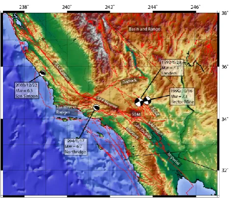
∼N 37◦W. While in Central California ∼80% of the mo-tion is taken up by the San Andreas Fault (SAF) (Prescott et al., 2001), in Southern California it is partitioned on dif-ferent faults, of which the SAF, the San Jacinto Fault (SJF), and the Elsinore Fault (ELS) are the most prominent ones. These three faults account for about 80% of the relative mo-tion (Bennett et al., 1996). This fault system consists of multiple segments, whose interaction is still not completely understood. The remaining 20% of the slip are accommo-dated offshore and along different fault systems further east, like the Eastern California Shear Zone (ECSZ) and the Basin and Range area (Fig. 1). In the past two decades four earth-quakesMw≥6.5 occured in the region, their location and
fo-cal mechanism1are also shown in Fig. 1. 3.2 Data
We used data provided mainly by two sources, the South-ern California Earthquake Center (SCEC) (Shen et al., 2003) and the Scripps Orbit and Permanent Array Center (SOPAC) (Jamason et al., 2004). The SCEC dataset is composed of ob-servations made with different geodetic techniques between
1from: USGS National Earthquake Information Center, http://
Fig. 1. Topographic map of Southern California with major faults.
Red lines indicate known faults and plate boundaries from: US Geo-logical Survey and California GeoGeo-logical Survey, 2006, Quaternary fault and fold database for the United States, accessed September 2008, from USGS web site: http://earthquakes.usgs.gov/regional/ qfaults/ and Michaud et al. (2004). SAF: San Andreas Fault, SBM: San Bernadino Mountains, ECSZ: Eastern California Shear Zone. Focal mechanism from USGS1.
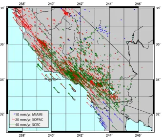
1970 and October 2001 (a full description is given by Shen et al. (2003)). The SOPAC dataset consists of continuous GPS measurements covering the time period from 1990 to 2008. It includes data provided by the Plate Boundary Observatory2 (PBO). To better allow for constraints on areas along the bor-der of our study region, we also included campaign observa-tions from the Eastern California Shear Zone (ECSZ) and Northern Baja collected and processed by the University of Miami (UM) (Dixon et al., 2002; Plattner et al., 2007, and P. LaFemina, personal communication, 2008) (see Table 1). In order to merge the different datasets, the SOPAC and UM data were rotated into the SCEC North America fixed ref-erence frame (RF), using the Eulerian pole that minimizes the residuals of the velocities at common sites (a list of com-mon sites and residuals is given in the Supplementary Ma-terial, see http://www.nat-hazards-earth-syst-sci.net/9/1177/ 2009/nhess-9-1177-2009-supplement.zip).
The final dataset consisted of 1261 velocity vectors within the area of interest in Southern California and adjacent re-gions (see Fig. 2). Note that all the data centers provided the velocities corrected for discontinuities in the time series (i.e. coseismic, instrumentation changes, and transient effects), providing long term interseismic velocities. This means that the strain map obtained from the data should be a represen-tation of the long term strain accumulation in the region.
2http://pboweb.unavco.org/?pageid=88
Table 1. Table of GPS velocity datasets used in the calculation.
Institution Number of sites used Sampling period
SCEC 769 1970–Oct 2001
SOPAC 991 1990–2008
UM 72 1994–2001
3.3 Strain rate tensor
Based on the distribution of the GPS observations, we tested different grid sizes to identify the best resolution. Too fine grid size results in a highly irregular strain rate map with high strain rate peaks at observation sites. It would be possible to increase the tensionT for the interpolation, but we noticed that such an interpolation introduces numerous artifacts. Too coarse grid size results in a very low and highly delocalized strain rate. The ideal situation would be to have a grid with at least one observation per cell. After different tests we found that a regular grid with cell size of 0.04◦, is most suitable for the interpolation of the horizontal velocity field compo-nents for Southern California. Using GMT routines (Wes-sel and Smith, 1991), we calculated the strain rate tensor as described in Sect. 2.2. The script used to produce the re-sults in this paper is attached in the electronic supplemen-tary material (see http://www.nat-hazards-earth-syst-sci.net/ 9/1177/2009/nhess-9-1177-2009-supplement.zip). Figure 3 shows the three components of the strain rate tensor. In or-der to avoid overinterpreting artifacts due to the interpolation scheme, we masked out (white color) interpolated values lo-cated at distances greater than∼0.5◦(15 grid cell) from near-est observation sites in all the figures.
This method is not suitable to calculate absolute values of strain rates. Since this value is related to the gradient of the velocity field, the rate is limited by the grid size, the mini-mal distance along which it is possible to observe a velocity change. Smaller grid sizes could overcome this problem, but they are associated with increasing uncertainties. However, the method is suitable to determine relative strain and strain rate changes.
3.4 Horizontal maximum shear strain rate
238˚ 238˚
240˚ 240˚
242˚ 242˚
244˚ 244˚
246˚ 246˚
32˚ 32˚
34˚ 34˚
36˚ 36˚
38˚ 38˚
238˚ 238˚
240˚ 240˚
242˚ 242˚
244˚ 244˚
246˚ 246˚
32˚ 32˚
34˚ 34˚
36˚ 36˚
38˚ 38˚
40 mm/yr, SCEC 20 mm/yr, SOPAC 10 mm/yr, MIAMI
Fig. 2. Map of Southern California with velocity arrows used in this study in a fixed North America reference frame. Red arrows: velocity
provided by the Scripps Orbit and Permanent Array Center (SOPAC); blue arrows: data from the University of Miami; green arrows: data from the crustal motion map (version 3) by the Southern California Earthquake Center (SCEC).
seismic hazards maps published by USGS3. This is essen-tially due to the fact that the “warm” color regions of Fig. 4 clearly reflect the location of the principal plate boundary between North America and the Pacific, following the major trace of the SAF. The maximum shear strain rate is highest in the south along the Imperial Fault and along the central sec-tion of the SAF (north of the Carrizo Segment). This can par-tially be a consequence of the fact that in these regions, the fault system is less complex, thus the deformation can bet-ter localize along the major segments of the fault. Probably, these high shear strain rates are related to the local aseismic creep of those segments of the SAF system. Creeping faults release part of the relative motion between the two sides by aseismic slip, implying that a large part of the deformation is accommodated on the fault plane in a really narrow region with very high shear strain rates. These do not necessarily correspond to high seismic hazard, since large parts of the deformation is not accumulated as elastic energy (B¨urgmann et al., 2001; Malservisi et al., 2005). Central Southern Cali-fornia is dominated by a more complex structure of slip par-titioning, which is also reflected in broader zones of rela-tively high shear strain rates, extending from the ECSZ to the Transverse Ranges.
3see e.g.: http://earthquake.usgs.gov/research/hazmaps/
products data/2008/
238˚ 240˚ 242˚ 244˚ 246˚
32˚ 34˚ 36˚ 38˚ 238˚ 240˚ 242˚ 244˚ 246˚
32˚ 34˚ 36˚ 38˚ 238˚ 240˚ 242˚ 244˚ 246˚
32˚ 34˚ 36˚ 38˚ 238˚ 240˚ 242˚ 244˚ 246˚
32˚ 34˚ 36˚ 38˚ 238˚ 240˚ 242˚ 244˚ 246˚
32˚ 34˚ 36˚ 38˚ 238˚ 240˚ 242˚ 244˚ 246˚
32˚ 34˚ 36˚ 38˚
−2.0 −0.5 0.0 0.5 2.0
µstrain/yr
ε.ee
εnn .
εen .
Fig. 3. Continuous symmetric strain rate tensor components
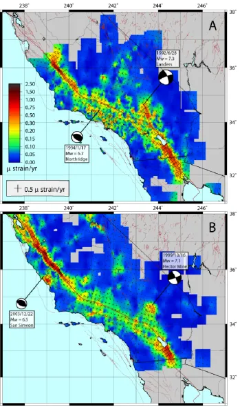
Fig. 4. Map of Southern California with magnitude (see colorbar) and direction (and its perpendicular, see black crosses) of maximum shear
strain rates. The size of the crosses is proportional to the magnitude of the maximum shear strain rate. Locations of observation sites are indicated by black circles and known faults (see Fig. 1) by brown lines. Values at a distance greater than 15 grid cells from any observation site are masked out.
At the transition between the Transverse Range region and the Imperial Valley, the map clearly shows that the maximum shear strain rate is partitioned between the SAF and SJF, with a minor contribution of the Elsinore Fault. The secondary plate boundary along the ECSZ/Walker Lane is also well vis-ible. This plate boundary separates the Sierra Nevada Block from the Basin and Range and accounts for about 11 mm/yr of relative motion (Dixon et al., 2000). The map shows rela-tively high shear strain rates in the Owens Valley region and at the south eastern part of the Mojave Region (probably due to recent large seismic events in the region). The Great Val-ley, which is characterized by low strain rates in the map, is essentially rigid and almost no deformation is observed.
Within the Great Valley some deformation is observed at lat-itude∼35.5◦N. Although it might be related to artifacts due to the lack of data, it is interesting to note that this region is intensively used for oil extraction. Wdowinski et al. (2007) already suggested that anomalous signals there may reflect data contamination by oilfield operations near Bakersfield. The two regions of deformation are also clearly visible as large subsiding areas in regional InSAR studies (F. Amelung, personal communication, 2008).
Fig. 5. Same as Fig. 4 using subsets of the data. (A) Map of the maximum shear strain rate based only on velocity data of SCEC collected
238˚ 238˚
240˚ 240˚
242˚ 242˚
34˚ 34˚
36˚ 36˚
238˚ 238˚
240˚ 240˚
242˚ 242˚
34˚ 34˚
36˚ 36˚
238˚ 238˚
240˚ 240˚
242˚ 242˚
34˚ 34˚
36˚ 36˚
−1.50 −1.00 −0.05 0.05 1.00 1.50
µstrain/yr
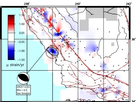
2003/12/22 Mw = 6.5 San Simeon
Fig. 6. Continuous dilatation rate field (see colorbar) of western
central California calculated from interseismic velocities, where negative values indicate compression and positive values extension. Black circles indicate site positions and brown lines known faults (see Fig. 1). Values at a distance greater than 15 grid cells from any observation site are masked out. The dilatation pattern reflects the focal mechanism of the San SimeonMw=6.5 earthquake on 22
December, 2003 (from USGS1). The high dilatation rates along the SAF are probably caused by creeping segments.
Simeon (2003,Mw=6.6) earthquakes. Apart from these
re-cent events, also large older earthquake seems to be still visi-ble in the dataset. In particular, we can note bright spot at the location of the 1872 (Intensity XI) Owens Valley and 1993 Eureka Valley (Mw=6.1) events. Since the velocities have
been corrected for coseismic displacement and for the short term post seismic deformation, it is likely that the observed high shear strain rates are related to visco-elastic relaxation. According to visco-elastic models (e.g. Savage and Lisowski, 1998), the surface velocity at a locked fault is highest right after an earthquake and decreases with time at a rate con-trolled by the local rheology. This transient behavior does not only explain why regions of recent seismic events appear much brighter, but also the relatively low rates at the SAF Mojave, the Transverse Range, and the Elsinore Fault that have not presented large seismic events in the past century and are supposed to be late in their earthquake cycles.
In order to test the interpolation and to analyze transient behavior, we performed a separate analysis of the data from SCEC and from SOPAC. As can be seen in Table 1, the two datasets include observations from different time spans (Fig. 5). In particular, the inclusion of data released by PBO within the SOPAC dataset allows for studying a more recent velocity field. A visual inspection of the two figures shows that it is not possible to do a full comparison of the two strain rate fields. The interpolation method is particular sensitive to site density, as high strain rates are directly related to big velocity changes within a narrow region. This becomes ap-parent in places like the LA Basin, where the SCEC dataset
is much denser than the SOPAC one. The method is also sensitive to the smoothing of the fields at the boundaries, as shown, for example, at the northern end of the SAF on the left and at the Imperial fault on the right. Thus, it is crucial to include observations for regions outside the one of interest (here: the inclusion of the data from UM or PBO data out-side Southern California) in order to reduce possible artifacts caused by edge smoothing.
Nevertheless, we note a considerable change of the maxi-mum shear strain rate between the maps in Fig. 5 in regions with comparable data distribution like the San Simeon area or the Landers/Hector Mine region. In the San Simenon region, the bright spot is present only in the SOPAC field. Since the 2003 earthquake happened after the release of the SCEC CMM v3 velocity field utilized here, the absence of the signal in the old strain rate field clearly indicates that the high shear is not associated with fault loading, but with post-seismic relaxation (see also next paragraph and Fig. 6).
In a similar way, we can observe that despite a similar coverage of geodetic observations, the maximum shear strain rate in the Landers/Hector Mine area is situated closer to the location of the Landers event for the SCEC data, and closer to the Hector Mine event for the SOPAC data. We relate this lo-cation shift of the maximum shear strain rate to the time span of the data collection in the two datasets. The postseismic re-laxation due to the 1992 Landers earthquake is clearly visible in the shear strain rate calculated using SCEC data only (see Fig. 5, A), whereas the high strain rates are probably related to postseismic effects of the 1999 Hector Mine and the 2003
Mw=6.5 San Simeon events which show up in Fig. 5 (B).
Un-fortunately, a similar analysis was not possible for the Owens Valley and Eureka Valley events, since the signal is mainly derived from episodic GPS observations conducted by the UM group and does not have different observation periods. A full study of the time series of the single GPS observations and the variation of the velocities with time is necessary to further investigate time dependent changes in the strain rate fields. Still, the comparison of the two strain rate fields shows that the method is also suitable for studying transient strain rates.
3.5 Dilatation rate
As a second example of the strain rate tensor analysis, we look at its trace. The sum of the diagonal elements of the tensor gives the rate of relative change of area (volume in 3-D) and provides the possibility to identify regions of com-pression or extension. Figure 6 shows an example of this analysis using only SOPAC data in the region of the San Simeon earthquake. As previously mentioned, the velocity field in this area is strongly influenced by postseismic visco-elastic relaxation and/or afterslip induced by the 2003 event. Indeed, the map of dilatation rate in the earthquake region reproduces the pattern of compression and extension of the published focal mechanism1. The highly localized dilatation pattern suggests that afterslip and not a broad-scale visco-elastic relaxation is the dominant postseismic mechanism. A dilatation rate pattern similar to the focal mechanism was also obtained for the Hector Mine earthquake. Using SCEC data only, we obtained a more complex dilatation rate pattern from postseismic deformation of the Landers event, which coincided quite well with Coulomb stress data modeled by King et al. (1994). The obtained patterns show the strength of the introduced method in the analysis of the transient be-havior of the strain rate and that the local velocity field is highly influenced by transient deformation probably induced by earthquake cycle effects.
At the northern end of the SAF in Fig. 6, we see that the di-latation rate shows a complex pattern. It is possible that this pattern reflects an artifact of the analysis. But it is worthy to note that this region corresponds to the transition between creeping and locked parts of the SAF and that the regional de-formation may be influenced by the local pattern of creep and transient deformation (Nadeau and Guilhem, 2009). Further-more, this is also the location of the 2004 ParkfieldMw=6.0
earthquake, which influences the local strain rate. A more detailed analysis of this pattern is beyond the scope of this work.
3.6 Coseismic strain
As a last example, we applied our method to a static dis-placement field instead of velocity data. The same interpola-tion method can be used to analyze a displacement field and results in strain instead of strain rate. It provides insights into the coseismic deformation, slip location, and rupture characteristics. We applied the method to the twoMw=6.5
andMw=6.4 earthquakes on 17 and 21 June, 2000 in the
South Iceland seismic zone, analyzing the displacement of 50 sites in South Western Iceland ( ´Arnad´ottir et al., 2001) (see Fig. 7). As expected by the strike slip nature of the two events, the rupture zones appear very clearly in a map of the maximum shear strain. The two bright spots in the map coin-cide with the location of the aftershocks recorded in the two
337˚ 337˚
338˚ 338˚
339˚ 339˚
340˚ 340˚
341˚ 341˚
63˚30' 63˚30'
64˚00' 64˚00'
64˚30' 64˚30'
300 mm
337˚ 338˚ 339˚ 340˚ 341˚
63˚30' 63˚30'
64˚00' 64˚00'
64˚30' 64˚30'
0.00 0.25 0.50 0.75 1.00 1.50 2.00 3.00 4.00 5.00 10.00
2*10−5 strain
10−5 strain
337˚ 338˚ 339˚ 340˚ 341˚
63˚30' 63˚30'
64˚00' 64˚00'
64˚30' 64˚30'
−5 0 5
10−5 strain
2000/06/21 Mw = 6.4
2000/06/17 Mw = 6.5
2000/06/21 Mw = 6.4
2000/06/17 Mw = 6.5
2000/06/21 Mw = 6.4
2000/06/17 Mw = 6.5
A
B
C
Fig. 7. Coseismic displacement (A), shear strain (B), and dilatation (C) caused by the two strike slip events on 17 June and 21 June,
weeks after the events4. Furthermore, the direction of the high shear zone is in good agreement with one of the planes of the focal mechanisms1. This suggests that the interpola-tion can clearly identify the region of the rupture.
The dilatation analysis shows that the far field has a very good agreement with the observed focal mechanism. The region between the two faults is clearly influenced by both events presenting a more complex pattern than the one ex-pected by the focal mechanisms. However, our geodesy based analysis can provide independent information for re-solving the rupture plain ambiguity of the focal mechanism solution.
4 Conclusions
Given the importance of strain accumulation on the earth-quake cycle, the study of regional strain rate is crucial for any seismic hazard assessment. Interpolation methods, as the one presented here, allow a derivation of the full tensor of strain rate from dense geodetic networks without the necessity to include any assumptions on the deformation mechanisms.
The analysis of the Southern California GPS data clearly shows that the method is capable to identify major regions of deformation. In particular, it indicates the importance of “secondary” plate boundaries like the Eastern California Shear Zone or the San Jacinto fault as regions of localized de-formation. This suggests the importance of studying the full diffuse boundary between the NA and Pacific plates in the analysis of deformation patterns. An analysis of the maxi-mum shear strain rate indicates that, apart from the LA basin, the direction of maximum shear is mainly controlled by the orientation of the SAF.
The strain rate map of Southern California also indicates a strong influence of transient effects. In particular, high strain rates are associated with regions of creeping, where the de-formation is strongly localized close to the fault plane, and with regions affected by postseismic deformation. Our anal-ysis of the SCEC and SOPAC data for Southern California clearly demonstrates that the postseismic deformation asso-ciated with past events is a strong component of the velocity field. An analysis of the evolution of the strain rate field is possible through the use of velocities derived from differ-ent periods. This analysis would provide important insight into the postseismic mechanism and rheological properties of the crust and the asthenosphere. The presence of localized strain rate associated with seismic events that did not hap-pen recently, like the Owens Valley or Landers earthquakes, indicates that the viscoelastic relaxation (e.g. Savage and Lisowski, 1998) has a strong impact on the observed geode-tic field. This transient behavior can create a major chal-lenge in the seismic hazard assessment. Current low strain
4from: Icelandic Meteorological Office, http://hraun.vedur.is/ja/
englishweb/earthquakes.html, accessed September 2008
rates at active faults cannot directly be related to low seis-mic hazard. At the contrary, the associated low strain rates can be an indication that the fault is late in its earthquake cy-cle, thus the rupture probability might be particularly high. On the other hand, bright spots in a strain rate map associ-ated with faults that recently experienced earthquakes could be related to a current low seismic hazard. Similarly, the high strain rates at creeping sections of a fault can be asso-ciated to lowseismic hazard. Thus, the strain rate map can contribute to seismic hazard assessment through the identi-fication of regions of localized deformation, but numerical modeling of the full lithospheric behavior, the seismic his-tory, and geological studies of the single faults are necessary in order to fully quantify the amount of elastic energy accu-mulated. Still, geodetically derived strain rate maps produce important geometric and regional constraints necessary for a correct modelling of the faults in the area. This analysis can also provide important information regarding the regions where more geological studies are necessary.
Finally, we would like to point out that the interpolation of geodetic data should not be limited to the study of velocity fields and associated strain rates, but can also be applied to other fields like coseismic displacement data. For example, the analysis of the coseismic strain derived from the observed displacements during the June 2000 earthquakes in Iceland indicates that the obtained strain tensor provides important insights into the location and direction of the events as well as information about the rupture.
Acknowledgements. We acknowledge the Southern California
Integrated GPS Network and its sponsors, the W. M. Keck Founda-tion, NASA, NSF, USGS, SCEC and SOPAC, PBO (UNAVCO) for providing data used in this study. We are grateful to Marleen Nyst and an anonymous reviewer for their careful reviews and Roland B¨urgmann and Christian Sippl for their comments. Thanks to the Icelandic Meteorological Office and Th´ora ´Arnad´ottir for the ice-landic data. This research was possible for the support of Munich Re and was partially funded by the DFG grant MA4163/1-1.
Edited by: M. E. Contadakis
Reviewed by: M. Nyst and another anonymous referee
References
Allmendinger, R. W., Reilinger, R., and Loveless, J.: Strain and ro-tation rate from GPS in Tibet, Anatolia, and the Altiplano, Tec-tonics, 26, TC3013, doi:10.1029/2006TC002030, 2007. ´
Arnad´ottir, T., Hreinsd´ottir, S., Gudmundsson, G., Einarsson, P., Heinert, M., and V¨olksen, C.: Crustal Deformation Measured by GPS in the South Iceland Seismic Zone Due to Two Large Earthquakes in June 2000, Geophys. Res. Lett., 28, 4031–4033, 2001.
Beavan, J. and Haines, J.: Contemporary horizontal velocity and strain rate fields of the Pacific-Australian plate boundary zone through New Zealand, J. Geophys. Res., 106, 741–770, 2001. Bennett, R. A., Rodi, W., and Reilinger, R. E.: Global
Position-ing System constraints on fault slip rates in southern California and northern Baja, Mexico, J. Geophys. Res., 101, 21943–21960, doi:10.1029/96JB02488, 1996.
B¨urgmann, R., Kogan, M., Levin, V., Scholz, C., King, R., and Steblov, G.: Rapid aseismic moment release following the 5 de-cember, 1997 Kronotsky, Kamchatka, earthquake, Geophys. Res. Lett., 28, 1331–1334, 2001.
Cai, J. and Grafarend, E. W.: Statistical analysis of geodetic defor-mation (strain rate) derived from the space geodetic measure-ments of BIFROST Project in Fennoscandia, J. Geodyn., 43, 214–238, 2007.
Dixon, T. H., Robaudo, S., Jeffrey Lee, J., and Reheis, M. C.: Present-day motion of the Sierra Nevada block and some tectonic implications for the Basin and Range province, North American Cordillera, Tectonics, 14, 755–772, 2000.
Dixon, T., Decaix, J., Farina, F., Furlong, K., Malservisi, R., Ben-nett, R., Suarez-Vidal, F., Fletcher, J., and Lee, J.: Seismic cycle and rheological effects on estimation of present-day slip rates for the Agua Blanca and San Miguel-Vallecitos faults, north-ern Baja California, Mexico, J. Geophys. Res., 107(B10), 2226, doi:10.1029/2000JB000099, 2002.
Fernandes, R. M. S., Miranda, J. M., Meijninger, B. M. L., Bos, M. S., Noomen, R., Bastos, L., Ambrosius, B. A. C., and Riva, R. E. M.: Surface velocity field of the Ibero-Maghrebian segment of the Eurasia-Nubia plate boundary, Geophys. J. Int., 169, 315– 324(10), 2007.
Frank, F. C.: Deduction of earth strains from survey data, B. Seis-mol. Soc. Am., 56, 35–42, 1966.
Haines, A., Jackson, J., Holt, W., and Agnew, D.: Representing distributed deformation by continuous velocity fields, Institute of Geological and Nuclear Sciences – Science Report, 98/5, 1998. Jamason, P., Bock, Y., Fang, P., Gilmore, B., Malveaux,
D., Prawirodirdjo, L., and Scharber, M.: SOPAC Web site (http://sopac.ucsd.edu), GPS Solutions, 8, 272–277, doi:10.1007/s10291-004-0118-2, 2004.
Jimenez-Munt, I., Sabadini, R., Gardi, A., and Bianco, G.: Active deformation in the Mediterranean from Gibraltar to Anatolia in-ferred from numerical modeling and geodetic and seismological data, J. Geophys. Res., 108, 2006, 2003.
Kahle, H.-G., Cocard, M., Peter, Y., Geiger, A., Reilinger, R., Barka, A., and Veis, G.: GPS-derived strain rate field within the boundary zones of the Eurasian, African, and Arabian Plates, J. Geophys. Res., 105, 23353–23370, 2000.
King, G. C. P., Stein, R. S., and Lin, J.: Static stress changes and the triggering of earthquakes, B. Seismol. Soc. Am., 84, 935– 953, 1994.
Kreemer, C., Haines, J., Holt, W. E., Blewitt, G., and Lavallee, D.: On the determination of a global strain rate model, Earth, Planet. Space, 52, 765–770, 2000.
Malservisi, R., Gans, C., and Furlong, K.: Microseismicity and Creeping Faults: Hints from Modeling the Hayward Fault, California (USA), Earth Planet. Sci. Lett., 234, 421–435, doi:10.1016/j.epsl.2005.02.039, 2005.
McGuire, R. K.: Computations of seismic hazard, Annals of Geo-physics, 36(3–4), 1993.
Michaud, F., Sosson, M., Royer, J.-Y., Chabert, A., Bourgois, J., Calmus, T., Mortera, C., Bigot-Cormier, F., Bandy, W., Dyment, J., Pontoise, B., and Sichler, B.: Motion partitioning between the Pacific plate, Baja California and the North America plate: The Tosco-Abreojos fault revisited, Geophys. Res. Lett., 31, L08604, doi:10.1029/2004GL019665, 2004.
Muir-Wood, R.: From global seismotectonics to global seismic haz-ard, Annals of Geophysics, 36(3–4), 1993.
Nadeau, R. M. and Guilhem, A.: Nonvolcanic Tremor Evolution and the San Simeon and Parkfield, California, Earthquakes, Sci-ence, 325, 191–193, doi:10.1126/science.1174155, 2009. Plattner, C., Malservisi, R., Dixon, T. H., Lafemina, P., Sella, G.
F., Fletcher, J., and Suarez-Vidal, F.: New constraints on relative motion between the Pacific Plate and Baja California microplate (Mexico) from GPS measurements, Geophys. J. Int., 170, 1373– 1380, doi:10.1111/j.1365-246X.2007.03494.x, 2007.
Prescott, W. H., Savage, J. C., Svarc, J. L., and Manaker, D.: De-formation across the Pacific-North America plate boundary near San Francisco, California, J. Geophys. Res., 106, 6673–6682, doi:10.1029/2000JB900397, 2001.
Reid, H. F.: The mechanics of the earthquake: the California earth-quake of April, 18, 1906, Report of the State Investigation Com-mission, v.2, Tech. rep., Carnegie Institution of Washington, 1910.
Savage, J. C. and Lisowski, M.: Viscoelastic coupling model of the San Andreas Fault along the big bend, southern California, J. Geophys. Res., 103, 7281–7292, 1998.
Shen, Z.-K., Jackson, D. D., and Ge, B. X.: Crustal deformation across and beyond the Los Angeles basin from geodetic mea-surements, J. Geophys. Res., 101, 27957–27980, 1996. Shen, Z.-K., Agnew, D. C., King, R. W., Dong, D., Herring, T. A.,
Wang, M., Johnson, H., Anderson, G., Nikolaidis, R., van Dom-selaar, M., Hudnut, K. W., and Jackson, D. D.: SCEC crustal motion map, version 3.0, online available at: http://epicenter.usc. edu/cmm3/ (last access: September 2008), 2003.
Smolka, A.: Schadenspiegel – Special feature issue Risk factor of earth, Tech. rep., Munich Re, 2007.
Spakman, W. and Nyst, M.: Inversion of relative motion data for estimates of the velocity gradient field and fault slip, Earth Planet. Sci. Lett., 203(15), 577–591, doi:10.1016/S0012-821X(02)00844-0, 2002.
Wdowinski, S., Sudman, Y., and Bock, Y.: Geodetic detection of ac-tive faults in S. California, Geophys. Res. Lett., 28, 2321–2324, doi:10.1029/2000GL012637, 2001.
Wdowinski, S., Smith-Konter, B., Bock, Y., and Sandwell, D.: Dif-fuse interseismic deformation across the Pacific-North America plate boundary, Geology, 35, 311–314, doi:10.1130/G22938A.1, 2007.
Wessel, P. and Bercovici, D.: Interpolation with Splines in Tension: A Green’s Function Approach, Math. Geol., 30, 77–93, 1998. Wessel, P. and Smith, W. H. F.: Free software helps map and display