A Probabilistic Estimation of the Basic Reproduction Number: A Case of Control Strategy of Pneumonia

Published online April 20, 2014 (http://www.sciencepublishinggroup.com/j/sjams) doi: 10.11648/j.sjams.20140202.12

A probabilistic estimation of the basic reproduction

number: A case of control strategy of pneumonia

Ong’ala Jacob Otieno

1

, Mugisha Joseph

1

, Oleche Paul

2 1

School of Mathematics, Statistics and actuarial Science, Maseno University, Kisumu, Kenya 2

Department of Mathematics, Makerere University, Kampala, Uganda

Email address:

[email protected] (Ong’ala J. Otieno), [email protected] (M. Joseph), [email protected] (O. Paul)

To cite this article:

Ong’ala Jacob Otieno, Mugisha Joseph, Oleche Paul. A Probabilistic Estimation of the Basic Reproduction Number: A Case of Control Strategy of Pneumonia. Science Journal of Applied Mathematics and Statistics. Vol. 2, No. 2, 2014, pp. 53-59.

doi: 10.11648/j.sjams.20140202.12

Abstract:

Deterministic models have been used in the past to understand the epidemiology of infectious diseases, most importantly to estimate the basic reproduction number, Ro by using disease parameters. However, the approach overlooks variation on the disease parameter(s) which are function of Ro and can introduce random effect on Ro. In this paper, we estimate the Ro as a random variable by first developing and analyzing a deterministic model for transmission patterns of pneumonia, and then compute the probability distribution of Ro using Monte Carlo Markov Chain (MCMC) simulation approach. A detailed analysis of the simulated transmission data, leads to probability distribution of Ro as opposed to a single value in the convectional deterministic modeling approach. Results indicate that there is sufficient information generated when uncertainty is considered in the computation of Ro and can be used to describe the effect of parameter change in deterministic models.

Keywords:

Basic Reproduction Number, MCMC, Pneumonia Model, Uncertainty, Sensitivity Analysis

1. Introduction

Pneumonia is a disease characterized by an inflammatory condition of the lungs and is caused by either bacteria, fungi, parasites or viruses. A high proportion of cases of pneumonia is reported to be caused by bacteria [25,37] especially Streptococcus Pneumoniae [5,9,16]. An individual can be infected by pneumonia if he/she inhales small droplets of coughs or sneezes containing the bacteria. Others carry the bacteria in their mouth or flora of nasopharynx without causing any harm [9,14,25] (we refer to them as carriers). However, the carriers do not get infected until the bacteria find its way into the lungs [7,14]. This is possible when the immunity of the individual is compromised.

Once the bacteria enter the lungs, they settle in the alveoli and passages of the lung where they rapidly grow and multiply in number. The invaded area of the lung then get filled with fluid and pus as the body attempts to fight off the infection [14]. This makes breathing difficult, painful and limits the intake of oxygen. Studies indicate that the risk factors that are associated with the spread of pneumonia include: malnutrition, lack of exclusive

breastfeeding, indoor pollution, antecedent viral infection amongst others [5, 16].

Deaths due to pneumonia can occur within three days of illness and therefore a prompt recognition and treatment with an effective drug is crucial. The treatment of pneumococcal diseases has been successful by use of antibiotics such as: penicillin, chloramphenicol for children and erythromycin for those patients who are allergic to penicillin [2,10]. However, a number of studies have indicated that the bacterium develops penicillin resistance [2, 22, 10]. Other antibiotics that have been used successfully are: amoxicillin and co-trimoxazole which are equally effective for non-severe pneumonia [2]. Over the last decade, there has been a significant impact on the empiric treatment of infections caused by Streptococcus Pneumoniae due to the substantial increasing trend of its resistance to antibiotic drug [37]. The drug-resistant strains contribute up to 35 percents of pneumonia cases [17] resulting to high number of deaths in many parts of the developing world.

90% since it’s inclusion in the national immunizations programs [10]. Two more vaccines for pneumonia (a 23-valent polysaccharide for adults and a 7-valent protein-conjugated polysaccharide for children) have also been in use since in 1983 and 2000 respectively [10,30] despite substantial argument over their efficacy [30]. A new 13-valent pneumococcal polysaccharide-protein conjugate vaccine (PCV13 [Prevnar13]) was licensed in 2010 to cover for more serotype [20]. Studies show that pneumonia cases have been reduced by 20% when vaccination is used, however it is faced with a number of challenges of resistance that is always developed by the bacteria. Major development of the vaccines against the bacteria is also proportional to the challenges but yet only 23 strains are covered in the current vaccine programs.

Pneumonia is infectious and is known to be one of the leading causes of morbidity and mortality in the developing countries with approximately 1.9 million people dying of the disease per year [33] translating to 4 individuals dying per minute in the developing countries due to pneumonia. Despite the increasing focus to reduce mortality in the developing countries arising from the Millennium Declaration and from the Millennium Development Goal 4 of United Nation-MDG [37], the under-five mortality rate has generated renewed interest in the development of more accurate assessments of the number of deaths of individuals aged less than 5 years. Moreover, monitoring the coverage of interventions to control these deaths has become crucial if MDG 4 is to be achieved [16]. Thus it is crucial to establish more accurate predictions of the causes of such deaths during the period of the first 5 years of living.

Mathematical models of infectious diseases have been used to successfully explain the transmission dynamics of many diseases and the use of such models have grown exponentially from mid 20th century [39]. A mathematical model for the transmission dynamics of streptococcus infection was previously developed by Doura et. al [24] and Ong’ala et. al [23]. However, their models neither incorporated control strategies nor used probabilistic approach in their simulation.

Probability modeling utilizes presumed probability distribution of certain input assumption to calculate the implied probability distribution of chosen output. We make use of Monte Carlo simulation technique to simulate the basic reproduction number of pneumonia dynamics. The values of the parameters are sampled from assumed probability distribution chosen as the basis for understanding the behavior of the parameter [28]. This approach of modeling has been described earlier in different studies viz: Uncertainty and Sensitivity Analysis of the Basic Reproductive Rate: Tuberculosis as an Example [29] and The Basic Reproduction Number in SI Staged Progression Model: A Probabilistic Approach [19].

2. Derivation of the Model

The model considers the transmission dynamics of

pneumonia in a population divided according their disease status of six compartments (Susceptible, Vaccinated, Infected, Carriers, Treatment and Recovered). The susceptible population can be increased by new recruitment of individuals through either birth or immigration at a constant rate . A proportion of susceptible that moves to the vaccinated class when they receive a vaccine against the disease is . The vaccine is expected to protect an individual from getting infected by the bacteria, however there is a possibility of the vaccine to wane [20] at the rate (where 1 − is vaccine efficacy) exposing vaccinated individuals to infections. The susceptible can be infected by either carriers or by symptomatically infected individual with a force of infection . The force of infection of a vaccinated individual is = , where is the proportion of the serotype not covered in the vaccine. A newly infected individual can either become a carrier with a probability or show disease symptoms with a probability (1 − ). The carriers can develop disease symptoms and become symptomatically infectious [13] at a rate or recover to gain immunity against the bacteria at an average rate . Therapeutic treatment can be applied to the infected at the rate . The rate of transfer from treatment class is denoted by . The transfer out of the treatment class is due to movement to recovery class if the treatment is effective or movement to infected class if the treatment is ineffective. The proportion of individuals for whom treatment is effective is denoted by . When treatment is applied, we assume that bacteria will be cleared and therefore the rate of transfer from the symptomatically infected class to the carrier class is negligible. The transfer rate from the infected individuals on the other hand can recover at a per capita rate of or die from the disease at a rate . We also assume that if treatment strategy is used, the infected individuals can’t move to the carrier class. The rate of losing the immunity is denoted by so that the recovered individual moves to the susceptible again. We denote the natural per capita mortality rate by μ. Using the variables and parameter described here, we generate the systems of differential equations for the model as in (2.1).

( )

( )

(1 ) (1 ) (1 ) ( )

( )

( )

( )

ds

v R V dt

dv

S V

dt dI

S V C T I

dt dT

I T

dt dC

S V C

dt dR

T C R

dt

δ ω λ ϕ µ

ϕ µ ω ελ

ρ λ ρ ελ π τ ϑ µ α ξ

ξ µ ϑ

ρλ ρελ µ π β

τϑ β µ δ

= + + − + +

= − + +

= − + − + + − − + +

= − +

= + − + +

= + − +

(2.1)

We define the force of infection λ as:

(I C) : k N

ε

λ = Ψ + Ψ = Ρ (2.2)

compartment, is contact rate and is the probability that a contact is effective to cause an infection. In this model, the total population at time is expressed as;

( )t ( )t ( )t ( )t ( )t ( )t ( )t

N =S +I +C +V +T +R (2.3)

For biological reasons, we assume that all state variables are more than or equal to zero a any time hence (2.1) has the initial conditions given by;

(0) (0) (0)

(0) (0) (0)

0, 0, 0,

0, 0, 0

S V C

T R N

≥ ≥ ≥

≥ ≥ ≥

From (2.3), boundness of solutions can easily be proven. Since;

( ) ( ) ( ) ( ) ( ) ( ) ( )

0 N_t S_t I_t C_t V_t T_t R_t

ν

µ

≤ = + + + + + ≤

Then, any variable of {N_{( )t} ,S_{( )t} ,I_{( )t} ,C_{( )t} ,V_{( )t} ,T_{( )t} ,R_{( )t} }

lies in the range 0, !.

System of equations in (2.1) is then studied in a suitable region:

6

{( , , , , , )S V I C T R R :N t( )

ν

}

µ

+

Ω = ∈ ≤

Thus " is a positively invariant and it is sufficient to consider solutions starting in " to remain in ". Therefore " is biologically feasible region and hence hence 2.1 is mathematically posed.

3. Analysis of the Model

For easier computation and analysis of (2.1), we use proportions instead of the population sizes The proportion of each variable can be obtained by dividing the class population sizes by the total population to get:

( ) ( ) ( ) ( ) ( ) ( )

, , , ,

( ) ( ) ( ) ( ) ( ) ( )

S t v t I t C t T t R t

s v i c f and r

N T N T N T N T N T N T

= = = = = =

Then by differentiating fractions with respect to time and simplifying, we have;

(1 ) ( )

ds v

s r v is i c s

dt = N − +δ +ω +α − Ψ + Ψ +ε ϕ

The rest of the rates of change of proportion are determined in the same way. Therefore by substituting # = 1 − $ − % − & − ' − at steady state of (2.1) we have;

(1 ) ( )

(1 )( )((1 ) ) (1 ) ( ) 2

( )

( )((1 ) ) ( )

( )

dv

r v i c f vi i c i v

dt di

i c r v i c f v c f i i i

dt df

i t if dt

df

i c r v i c f v i ic

dt dr

f c i r ir

dt

ϕ

α

ω

ε

µ α

ρ

ε

π

τ ϑ

α ξ µ α

α

ϑ µ α

α

ρ

ε

π β µ α

α

τϑ

β

µ α

δ

α

= − − − − − + − + ∈ Ψ + ∈ Ψ + +

= − Ψ + Ψ − − − − − + ∈ + + − − + + + +

= + + +

= Ψ + Ψ − − − − − + ∈ − + + + +

= + − + + +

(3.1)

The system (3.1) can now be studied in ( = {(%, ', &, *, $)}. All the solutions of system (3.1) are positively invariant in Γ. Consider the first equation in system (3.1)

(1 ) ( )

( )

dv

r v i c f vi i c i v dt

dv

v dt

ϕ α ω ε µ α

ϕ ϕ ω µ

= − − − − − + − + ∈ Ψ + ∈ Ψ + +

≤ − + +

Solving for v(t) gives

( )

0

( ) t

v t

ϕ

v e ϕ ω µ

ϕ ω µ

− + +

≤ +

+ + (3.2)

As t → ∞ we obtain 0 ≤ v(t) ≤ 1

Similar proof can be established for '( ), &( ), *( ) and $( ). Hence all feasible solutions of system (3.1) starting in

( remains in ( where;

6

{( , , , , )

,

, , ,

0}

1

v c i f r

R

v c i r

and v c i

f

r

Γ =

∈

≥

+ + + + ≤

3.1. Basic Reproduction Number

We use the next generation approach to determine the basic reproduction number of (3.1). Let 1₂ be the rate of appearance of new infections into the compartment and

i i i

eigenvalue) of the matrix 1359as;

( )(( )( ) ( ) + ))

( )( ) ( )( )( )

Rvt µ ϕ ω µ ϑ µ µρ π β ρβ ρεϑ α µ ξτ µ α µ ξ

ϑ α µ ξτ ϕ ω µ µ α µ ξ ϕ ω µ π β µ

Ψ +∈ + + − + + − + + + + +

=

+ + + + + + + + + + +

（

(3.3)

3.2. Vaccination Effect on the Basic Reproduction Number

Assume there is no treatment, then (3.3) is written in two terms as;

{(1 )( ) } ( )}

[ ] [ ]

( )( )

v

R µ ϕ ω ρ π β µ ρπ ρε α µ

µ ϕ ω α µ π β µ

+ ∈ + − + + + + +

= Ψ

+ + + + + (3.4)

Equation (3.4) is defined as the basic reproduction number with vaccination alone. The first term corresponds to the vaccination parameter and can be expressed further as;

(1 )

[

µ

ϕ ω

] [

ϕ

]

µ ϕ ω

µ ϕ ω

+ ∈ + ₌ − ∈

+ + + +

Using (3.2), as → ∞ , ₀ ϕ ₁

µ ϕ ω

≤ ≤

+ + hence (1 )

0

ϕ

1

µ ϕ ω

−∈

≤ ≤

+ + since 0 ≤ ϵ≤1. Therefore,

(1 )

[1

ϕ

] 1

µ ϕ ω

−∈

− ≤

+ + (3.5)

The second term of (3.4) corresponds to the basic reproduction number, 6_E without control any control strategy as derived by [23]. Hence we have (3.4) expressed as;

0 (1 )

[1 ]

v

R

ϕ

R

µ ϕ ω

− ∈ = −

+ + (3.6)

From (3.5) and (3.6), it implies that 6 ≤ 6_E. When = 0 (implying that there is no vaccination), then 6 = 6E. The introduction of vaccination implies that

6 ≤ 6E, and consequently if 6E< 1, then 6 < 1 for

φ > 0.

3.3. Treatment Effect on the Basic Reproduction Number

Consider a case when treatment only is used as control strategy where φ = 0(no vaccination) then (3.3) is written as

t

( ){(1 )( ) }

[ ][ ]

( ) ( ) ( )

R µ ϑ ρ π β µ ρπ ρε

π β µ ϑ α µ ξτ µ α µ ξ

Ψ + − + + +

= +

+ + + + + + + (3.7)

Differentiating 6_G with respect to τ yields

t ₂

( )( )

( )( ( ) ( ))

R µ ϑ µ µρ π β ρβ ϑξ

π β µ ϑ α µ ξτ µ α ξ µ

Ψ + − + + −

=

+ + + + + + + (3.8)

Then 6G is a decreasing function with respect to ; implying that any increase in the treatment efficacy is a significant strategy for controlling the disease.

4. Probabilistic Simulating of the Basic

Reproduction Number

The basic reproduction number is defined as the expected number of secondary infections realized when an infected individual is introduced into a purely susceptible population. It is one of the most important concern parameter for a disease to invade a population [30]. It is clear that when the basic reproduction number is below one, each infected individual produces less than one newly infected individual on an average hence possibility of clearing the infection from the population. We determine which control measures and at what magnitude would reduce the Basic Reproduction number below one at a greater percentage by using Markov Chain Monte Carlo (MCMC) technique to simulate the variation of basic reproduction number.

The basic reproduction numbers 6 and 6_G given in (3.3) and (3.7) respectively are derived from a mathematical model that reflects the biology of the transmission dynamics of Pneumonia. The 6 is a function of 13 different parameters while 6_G is a function of 10 different parameters. When we compute the values of the basic reproduction numbers using single values of the parameters, then the result is a single value. Since each of the model’s parameters are uncertain, we consider the parameters to be random variable following different probability distributions then study the distribution of the basic reproduction number with the random effects of the parameters.

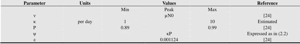
A probability density function is assigned to each parameter based on their possible values and probability of occurrence of any specific values. The possible values of the parameters are estimated from literature (see Table 1). The parameters with peak values are considered to follow approximately triangular probability distribution while those without peak values assumed to follow approximately uniform probability distribution.

Table 1. The model parameter values and assumed distributions: The Probability Distribution are either uniform (when the minimum and maximum values

are given) or triangular (when peak values are given..

Parameter Units Values Reference

Min Peak Max

ν µN0 [24]

κ per day 1 10 Estimated

P 0.89 0.99 [24]

ψ κP Expressed as in (2.2)

Parameter Units Values Reference

ρ 0.085 0.28 0.338 [26], [15]

π per day 0.00274 0.01096 [24]

η per day 0.0238 0.0476 [34]

α 0.15 0.33 Estimated

δ 0 0.3 Estimated

µ per day 0 0.00004793 0.0002 [39]

β 0 0.0115 0.0165 [32]

φ 0.7 0.8 0.9 [11]

ω 0.15 0.44 [3]

ϵ 0.2 0.48 0.76 [12]

τ 0.3 0.5 Estimated

ξ 0.43 0.56 0.78 [15]

5. Results

Monte Carlo Markov Chain simulation methods employ the most appropriate sampling scheme resulting into N = 10, 000 samples for each parameter. For each sample, the basic reproduction number (Ro, Rt, Rv and Rvt) are computed and their empirical probability values calculated when their value(s) is less than one and when more than one after from all the 10,000 sample (Table 2).

Table 2. The empirical probability values when the basic reproduction

number is less than one and when more than one.

Count Empirical Probability

<1 <1 >1

Ro 52 0.0052 0.9948

Rt 2889 0.2889 0.7111

Rv 3755 0.3755 0.6245

Rvt 4836 0.4836 0.5164

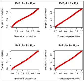
The histograms and probability distribution for Ro, Rvt, Rt and Rv are obtained as shown in Figure 1. The fitted probability distribution for the histograms in Figure 1 is approximation of the observed data whose parameters are given in Table 1 and their P-P plots illustrated in Figure 2.

Figure 1. Histograms and probability density functions of Ro, Rt, Rv and Rvt

of pneumonia model.

The best fit probability distributions for Ro, Rt, Rv and Rvt are shown in Table 3 which indicates that when no control strategy are used, the basic reproduction number is normally distributed with a mean of 5.60 and a standard deviation of 2.75. This means that any shift on the value of the mean to the right will propagate the disease positively and viceversa.

Table 3. Probability distributions with their parameters specified.

Distribution Parameters Estimates Mean Ro∼ N (µ, σ2 ) µ = 5.60, σ = 2.75 E(Ro )=5.60

Rt∼Γ(κ, β) κ = 1.7270, β = 0.8995 E(Rt )=1.9199

Rv ∼ Weib(κ, λ) κ = 1.363, λ = 1.7007 E(Rv )=1.556

Rtv ∼ Weib(κ, λ) κ = 1.4833, λ = 1.2686 E(Rtv )=1.149

The basic reproduction number when considering vaccination only in distributed according to Weibull with a shape parameter of 1.363 and a scale parameter of 1.7. When treatment strategy is applied, then the basic reproduction number is distributed according to gamma with shape parameters of 1.727 and rate parameter of 0.89. Finally, when both the treatment and vaccination strategy are used, then the basic reproduction number is distributed according to the Weibull with a shape parameter of 1.48 and a scale parameter of 1.27.

The value of the basic reproduction number R is a useful indicator because it helps to determine whether or not an infectious disease can spread through a population.

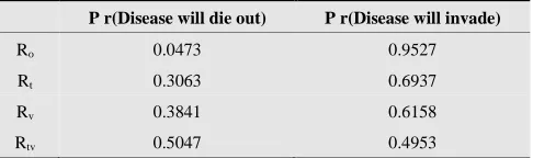
When 6 < 1 then the infection will die out in the long run. But if 6 > 1 then the infection will be able to spread in a population. Using the results in Table 3, we show in Table 4 that the probability that the infection will die out or spread in the population by computing P r(R ≤ 1) and P r(R > 1) respectively.

Table 4. Probability of disease inversion.

P r(Disease will die out) P r(Disease will invade)

Ro 0.0473 0.9527

Rt 0.3063 0.6937

Rv 0.3841 0.6158

Rtv 0.5047 0.4953

6. Conclusion

A quantitative analysis can be performed by using single-point estimates (referred to as deterministic). Using this method, one may assign values for discrete parameters to see what outcome they might have on the basic reproduction number from each. For example, what parameter values will result to a basic reproduction number of 1, less than 1 or more than 1. However, the approach considers only a few discrete outcomes, ignoring hundreds or thousands of others. It also gives equal weight to each outcome. That is, no attempt is made to assess the likelihood of each outcome.

Monte Carlo simulation is a better way of addressing the drawbacks where uncertain inputs in a model (basic reproduction number) are represented using ranges of possible values of known (or assumed) probability distributions. By using probability distributions, parameters can have different probabilities of different outcomes occurring. Probability distributions are a much more realistic way of describing uncertainty in parameters used in computing the basic reproduction number. Fitting the probability distributions remove any noise that may be available in your data hence improves the results. This explains the difference in Table 1 (probabilities computed from the simulated data) and Table 3(probabilities computed from the fitted probability distribution).

Acknowledgements

Many thanks to the reviewers and referees of their corrections to make this paper what it is now.

References

[1] A. Brueggemann, D.T. Griffiths, E. Meats, T. Peto, D.W. Crook and B.G. Spratt (2003), “Clonal Relationships between Invasive and Carriage Streptococcus pneumoniae and Serotype- and Clone-Specific Differences in Invasive Disease Potential”, The Journal of Infectious Diseases. Vol 9(187) pp. 1424-1432

[2] A. Brueggemann and V. G. Doern (2000), “Resistance Among treptococcus pneumoniae: Patterns, Mechanisms, Interpreting the Breakpoints”, The American Journal of Managed Care. Vol 6(23) pp.1189-1196.

[3] A. Kuhlmann, U. Theidel, M. W. Pletz and J Schulenburg1, (2012) “Potential cost-effectiveness and benefit-cost ratios of adult pneumococcal vaccination in Germany” Health

Economics Review.

http://www.healtheconomicsreview.com/content/2/1/4 2 4 [4] B. Ashby and C. Turkington (2007 ),, The encyclopedia of

infectious diseases 3rd Edition, Website Publication

-http://books.google.co.uk/ books?id

=4Xlyaipv3dIC/pg=PA242.

[5] B. Greenwood 354 (1999), “The epidemiology of pneumococcal infection in children in the developing world,” The Royal Society. Pp. 777-785

[6] B.M. Gray, G.M. Converse and J. Dillon (2007), “Epidemiologic Studies of Streptococcus pneumoniae in Infants: Ac-quisition, Carriage, and Infection during the First 24 Months of Life”, The Journal of Infectious Diseases Vol 3 .pp.142

[7] C. Davis (2010), “Pneumoniae”: Retrieved September 2011,

from Medicinenet.com, http://

www.medicinenet.com/pneumonia/article.htm 2howdo. [8] D. Kateete, H. Kajumbula, K. Deogratias and A. Ssevviri,

(2012), “Nasopharyngeal carriage rate of Streptococcus pneu-moniae in Ugandan children with sickle cell disease”, BMC Research Notes pp. 321-416

[9] D. Pessoa, (2010), “Modelling the daynamics of Streptococcus pneumoniae Transmmission in children” Masters thesis, University of De Lisboa.

[10] D. T. Jamison, (2006), “Disease control priorities in developing countries, Part 611 Stand Alone Series,” World

Bank Publications,

http://books.google.co.ke/books?id=Ds93H98Z6D0C 2 [11] GAVI, , (2011), “Statement of Alex Palacios on the Global

Alliance for Vaccines and Immunizations (GAVI) Alliance” [12] G. Aslan, G. Emekdas, M. Bayer, M. Sami, N. Kuyucu and A.

Kanik (2007), “Serotype distribution of Streptococcus pneumoniae strains in the nasopharynx of healthy Turkish children” Indian Journal of Medical research Vol. 125pp. 582-587

[13] G. McKenzie (1999), “The Pneumococcus Carrier”, The Mary Imogene Bassett Hospital pp. 88-100

[14] G. Schiffman and C. Melissa (2010), “Pneumonia”,

MedicineNet. Retrieved from

http://www.medicinenet.com/pneumonia/article.htm 2howdo ,

[15] H. Gazi, S. Kurutepe, S. Surucuoglu and A. Teker, (2004), “Antimicrobial susceptibility of bacterial pathogens in the oropharynx of healthy school children in Turkey.” Indian Journal of Medical research Vol. 120 pp. 489-494

[17] J. Anthony, G. Scott, W. Abdullah,P. Walik, H. Douglas and M. Kim (2008),, Pneumonia research to reduce childhood mortality in the developing world, Journal of Clinical Investigation. Vol 4(118) pp. 1291-1300

[18] J. Dushoff, W. Huang and C.Carlos, (1998), “Backwards birfurcations and catastrophe in simple model of fatal diseases”, Journal of Mathematical Biology Vol.36 pp. 227-248

[19] J. Kodaira and J. Passos(2010), “The Basic Reproduction Number in SI Staged Progression Model: A Probabilistic Approach”, International Conference on Chaos and Nonlioniear Dynamics

[20] J. Nuorti and C. Whitney (2010), “Prevention of Pneumococcal Disease Among Infants and Children Use of 13-Valent Pneumococcal Conjugate Vaccine and 23-Valent Pneumococcal Polysaccharide Vaccine, Division of Bacterial Diseases”, National Center for Immunization and Respiratory Diseases 59

[21] J. M. Heffernan, R.J Smith, and L.M Wahl (2005),, Perspectives on the basic reproductive ratio, Journal of the Royal Society Interface. Vol 4(2) pp. 281-293

[22] J. Starr, G. Fox and J. Clayton, (2008), “Streptococcus pneumoniae: An Update on Resistance Patterns in the United States”, Journal of Pharmacy Practice. Vol 5(21) pp. 363-370

[23] J. Ong’ala, J.Y.T Mugisha and P. Oleche, (2013), “Mathematical Model for Pneumonia Dynamics with Carriers,” Inter-national Journal of Mathematical Analysis, Vol 7 pp. 2457 - 2473

[24] K. Doura and D. Malendez-Morales and G. Mayer and L.E Perez, (2000), “An S-I-S Model of Streptococcal Disease with a Class of Beta Hemolytic Carriers”

[25] K. Todar (2011), “Streptococcus, Online Textbook of Biology”,

http://textbookofbacteriology.net/S.pneumoniae.html. [26] M. Bakir, A. Yagci, C. Akbenlioglu, A. Ilki, N. Ulger and G.

Syletir, (2002), “Epidemiology of Streptococcus pneumoniae pharyngeal carriage among healthy Turkish infants and children” European Journal of Pediatrics. Vol. 161 pp. 165-166

[27] M. Darboe, A. Fulford, O. Secka and A. Prentice(2010), “The dynamics of nasopharyngeal streptococcus Pneumoniae carriage among rural Gambian Mother-child pairs”, BioMed Central Infectious Diseases, Vol 95(10) pp. 1471-2334

[28] M. Pergler and A. Freeman (2008), “Probabilstic Modeling as an Exploratory decision Making tool”, McKinseyand Company, Working Paper

[29] M. Sanchez and S. Blower, (1997), “Uncertainty and Sensitivity Analysis of the Basic Reproductive Rate: Tuberculosis as an Example”, American Journal of Epidemiology. Vol. 12(145) pp. 1127-1137

[30] N. W. Schluger, (2006), “Vaccinations Bacterial, for Pneumonia, Encyclopedia of Respiratory Medicine”. Vol 5(21) pp. 389-392

[31] P. C. Appelbaum, (2003), “Resistance among Streptococcus pneumoniae: Implications for Drug Selection”, Oxford Jour-nals of Clinical Infectious Diseases. Vol 12(34), pp 1613-1620

[32] P. Hill, Y. Cheung, A. Akisanya, K. Sankareh, G. Lahai, B. Greenwood and R. Adegbola, (2008), “Nasopharyngeal Carriage of Streptococcus pneumoniae in Gambian Infants: A Longitudinal Study,” Clinical Infectious Disease Journal Vol 6 (46) pp. 807-814

[33] R.E. Black and S. Moris and J. Bryce (2003), Where and why are 10 million children dying every year, Lancet. Vol (361) pp. 2226-2234

[34] R. Thadani, (2011), “Pneumonia Recovery Time”, http://www.buzzle.com/articles/pneumonia-recovery-time.ht ml

[35] S. Cousens, E.R. Black, L. H. Johnson, I. Rudan, D. G. Bassani and R. Cibulskis, Global, (2010), “Regional, and national causes of child mortality in 2008: a systematic analysis”, Lancet. Vol 375 pp. 1969-1987

[36] S. Obaro and R. Adegbola, The pneumococcal: carriage, disease and conjugate vaccine, J Med Microbiol 2 (2002), 98-104

[37] United Nations, (2011), “Milleniam Development Goals,” United Nations website, http://www.un.org/millenniumgoals/ [38] World Health Organization(2010),, “Global Health

Observatory Data Repository”,

http://apps.who.int/ghodata/?vid=1320.

[39] W. Hethcote, (2000), “The Mathematics of Infectious Diseases”, Society for Industrial and Applied Mathematics Vol. 424 pp. 599-653