Large-Scale Systems Control Design via LMI Optimization
Branislav Rehák
Institute of Information Theory and Automation, Pod Vodárenskou, věží 4, 182 08 Praha 8, Czech Republic,
e-mail: [email protected]
http://dx.doi.org/10.5755/j01.itc.44.3.6464
Abstract. A control design for a large-scale system using LMI optimization is proposed. The control is designed in a way such that the LQ cost in the case of the decentralized control does not exceed a certain limit. The optimized quantity are the values of the control gain matrices. The methodology is useful even for finding a decomposition of the system, however, some expert knowledge is necessary in this case. The capabilities of the algorithm are illustrated by two examples.
Keywords: combinatorial linear matrix inequalities, large-scale system, decentralized control.
1. Introduction
Control of large-scale complex systems has gained great attention long time ago. This is due to its sheer practical importance as well as due to the many theoretical problems emerging from this area. First, algorithms for decentralized control of complex systems have been proposed. As an example, [1] proposes a decentralized control of linear systems minimizing a quadratic cost functional. Recently, we have witnessed a new interest in the decentralized control. This can be also granted to the fact that new computational methods opened up further possibilities for applications of new hierarchical and decentralized control strategies. They often require a larger amount of computational effort. Some recent trends are summarized in [2]. A series of results concerning decomposition of optimal control problems and calculus of variations can be found in [3,4].
A related problem is the problem of decomposition of large systems into subproblems. This problem has been solved using the graph theory in [2] and [5]. Theory of fixed modes [6] is another way how to attack this problem. Roughly speaking, fixed modes are modes in the closed loop that cannot be modified under decentralized feedback which is assumed to have a predefined structure. A method that allows us to overcome this disadvantage is presented in [6]. This method is based on the solution of several linear matrix inequalities (LMI) such that a certain objective function is minimized. The minimized quantity is the square of the elements in the feedback matrix corresponding to the interconnections. Hence this
algorithm allows us to find a control that minimizes the amount of information exchanged during the control process.
Early results about control of large-scale systems were obtained in the seventies. From those times, a large number of papers emerged treating the decomposition problem from various angles. We provide only an incomplete selection of several papers that were inspiring for the presented work.
Decomposition problem using graph-theoretic methods have been proposed, for example the decomposition (see [7], further results can be found e.g. in [8]). In this approach, one seeks for a permutation of rows and columns so that the system matrix after this transformation has "almost" block-diagonal structure. This means, all off-block-diagonal blocks have the norm less than ε. Decomposition of a system with overlapping structure using the inclusion principle is presented in [9]. Dynamical programming coupled with graph-theoretic considerations is used for system decomposition in [10].
Stochastic large-scale systems are an important extension of large-scale systems. In this case, one has to investigate the effects of random noise to stability of interconnected systems.
Ferreira et al. study conditions for stability (especially stochastic stability and noise-to-state stability) of interconnected stochastic systems in [11].
There are many applications of decomposition theory. Let us mention examples in biology which include [14,15], control of unmanned aerial vehicles is proposed in [16], for applications to power networks safety see [17].
Application of linear matrix inequalities was presented in several papers recently. A robust control problem involving decomposition of a system and finding a control for a decomposed system using linear matrix inequalities is solved in [18], [19] or [20], however, treating off-diagonal entries is different than in this paper. Especially, the approach adopted here allows finding a control even for the case when the interconnections do not allow using purely decentralized control. Recent optimization technique, namely the sum-of-squares, is applied for decomposition of large systems in [21]. This paper also presents an application to a biological system - a model of the Epidermal Growth Factor signalling pathway.
So far, the algorithms to solve the decomposition problem were designed so as the computations could be done for separate subsystems. However, with the rise of computational power and also with advent of efficient algorithms, one does not need to handle the subsystems separately. Rather, one can deal with the whole system in the control design phase. One of the efficient algorithms is also the convex optimization (see [22] for details) and solving the LMIs as shown in [18, 21], dynamic output feedback control for large scale systems designed using LMIs is presented in [23]. One can employ algorithms that use convex optimization of large problems. Presenting a method that makes use of capabilities of the modern computer technology, especially handling large LMI problems, is one of contributions of this paper. One such decomposition method based on solution of a large convex optimization problem is presented in [24] and, in an extended form, in [25]. There, a cost of the optimal control disregarding the need for the decentralization was computed. Then, a decentralized controller was sought such that the cost caused by using this controller does not exceed some predefined bound which was selected using the cost of the centralized LQ-optimal control. If this control is not achieved, some interconnections are allowed and the computation is run once again. To our best knowledge, this approach to decentralized control has not been studied before.
Instead of the LQ-optimal control, robust control is used. This is due to the fact that its use brings some other advantages. The first and most important is that the inaccuracies caused by neglecting some terms (mainly nondiagonal) can be treated as uncertainties and, consequently, stability of the whole control loop can be tested.
The aim of the paper is to introduce another method for decentralized control design. This method is also applicable for finding of a control structure in the case that a fully decentralized control cannot be
found. Another important feature is that the quadratic cost of the decentralized control does not exceed the cost of a centralized LQ control by more than a prescribed margin.
The novelty of the approach adopted in this paper is that the values of the control gain matrix are the optimized quantity. The LQ cost is regarded as an auxiliary variable and plays the role of a constraint. The formulation of the LMI optimization problem is rather non-standard, however, it allows to easily find the desired control. To the author's knowledge, a similar approach was not used before. Also, the interconnections may have an arbitrary structure.
The method is based on linear matrix inequalities (LMI) and makes use of the fact that solvers for solution of this problem are now available and work reliably even a large problem is solved. Hence there is no need to restrict the size of the computational load in the phase of control design. This contrasts with the requirement of decentralized control law as the centralized control might still be impossible or impractical to apply.
The layout of this paper is standard. After this introduction, the problem is defined. After that, the solution of the problem using LMIs is formulated so that this algorithm is ready-to-use then. A set of examples follows together with some remarks about practical implementation.
2. Algorithms
Stabilization
Let N be a positive integer. For each i=1,...,N we define positive integers ni, mi. Assume matrices Ai ( ni-dimensional), AD (n-dimensional), Bi, (dimension ni x mi) and BC (n x m-dimensional) are given. Here, n=n1+...+nM, m=m1+...mN. The interconnected system is given by
x
A
x
A
A
x
CN
0
0
1
(1)
u.
B
+
u
B
B
+
CN
0
0
1
The system
i i i i i=Ax+Bu
x (2)
is called the i-th subsystem.
The interconnected system can be seen as the set of subsystems interconnected by the matrices AC, BC. In the following section, if we speak about subsystems, we will always think about them as parts of the interconnected system (1).
are supposed to be positive semidefinite, the matrices Ri are positive definite. Then, using
N
N R
R R Q Q
Q
0
0 ,
0
0 1
1
one can define the cost functional
t Qxt +u Ru
t dt. xJ
T
0
(3)
The goal is to design a controller in the form u=Kx where the matrix K has a decentralized structure. Ideally, the nonzero elements should be placed so that the structure of the system given by the matrices AC,
BC remains. This might be possible. However, in some
cases, the matrix K should have nonzero entries on other positions to achieve stability. The number of these elements should be minimized. Another objective is to find the controller so that the increase of the cost defined by the cost functional is not large (a more precise explanation is given later).
The controller design can be described now. First, one computes the centralized LQ controller for the interconnected system. The solution of the corresponding Riccati equation is denoted by PC. If the initial condition of the system (1) is x(0) then the optimal cost in the case of centralized LQ control is J=xT(0)PCx(0). In general, this cost cannot be achieved under the decentralized control law, however, our aim is to design a control such that
) 0 ( ) 0 ( ) 0 ( ) 0
( P x sx x
x
J C T
T
D (4)
for a given s>0. Using [26], the value of the functional (3) is given as J=xT(0)PDx(0) where the symmetric positive definite matrix PD satisfies the equation
RK K Q
BK A P P BK A
T D D T
) ( )
( (5)
provided the control is given by u(t)=Kx(t). Using the above considerations, the condition (4) can be reformulated as
sI
P
P
D
C
(6)where I is the identity matrix of a suitable dimension. Let us turn our attention to the definition of the weighting matrices that allow us to choose some elements of the matrix K to be rendered to zero. Let gij>0. Using this, one can define the objective
function.
N N
m m
i
n n
j
ij ij
k
g
Minimize
1 1
1 1
2
).
(
(7)Minimization of this function is described in the following section.
Reference tracking
In this case we assume that the reference is generated by an autonomous system, the reference generator. The output of this reference generator must coincide with the output of the system which is also to be defined yet.
Let the positive integers p1,...pN be given. Assume the output of the i-th subsystem is given by
. n R C , x C =
y pi i
i i i i
Define also C=diag(C1,...CN). To be able to design a decentralized controller, the reference generator must be in a decentralized form itself. It is defined by the equation
Sq r Mq =
q , (8)
where M=diag(M1,...MN), S=diag(S1,...SN), Mi are μi -dimensional square matrices and Si have dimension pi x μi. The reference is determined by the initial condition q(0).
The goal is to design matrices K, Kr having suitable dimensions such that the condition
t r t 0x
holds (for t increasing) under the control law
t. q K + t Kx tu() () r
Moreover, the structure of the matrices K, Kr must also meet the decentralization requirements.
The decomposition of the reference generator seems to be superfluous. However, to design a decentralized control scheme, the decentralized structure even in the reference generator is crucial.
Define Ar=diag(AC,M), Br=(BCT,0)T, Cr=(CC,-S).
Using these definitions, one can introduce the augmented system
.
,
r
x
x
u
B
x
A
x
r r r r r (9)Finally, define the matrix Qr by Qr=CrCrT+aI with a parameter a>0 guaranteeing regularity of the matrix Qr.
In the following text, one works with the system (9) as in the previous case. The matrices Ar, Br etc. play the role of matrices A, B in the previous section, respectively.
3. LMI formulation of the optimization
problem
Note that the minimization problem is not convex due to the multiple of matrices PD, K in (5). The way how to recover the convex structure of the problem is presented in this section.
If PD>0, then one defines QD=PD-1 (note that QD>0
as well). Multiplying the equation (5) by QD from both sides and denoting
Y=K QD (10)
yields
RY Y +
QQ Q < BY + B Y + AQ + A Q
T
D D T
T D T
D
which can be, using the Schur complement, rewritten into the form
0 0
0
1
1
R Y
Q Q
Y Q Z
D
T D
(11)
where
BY. B Y AQ A Q =
Z T T
D T
D
The inequality (6) yields
. ) ( 1
P sI
QD C (12)
Let us turn our attention to the objective function (7) whose value is to be minimized. Note that (10) implies that the values of kij are given as elements of the matrix QD-1Y. Hence, (7) is reformulated using
elements of the matrices QD and Y.
The way how the variable Y was defined hints that absolute value of certain elements of the multiple QD-1 must be minimized. However, elements of this
expression cannot be easily extracted without breaking convexity of the problem. Hence the objective function is modified in the following way: the elements of the matrices Y and QD are penalized separately.
To minimize the undesired terms of the matrix Y an objective function is defined. Minimization of this objective function implies minimization of these terms. The matrix Y is expressed as
.
Y
Y
=
Y
dD
nDThe decomposition of the matrix Y is carried out as follows: let (i,j) be such that the element kij should be penalized. Then (YdD)ij=0. Conversely, if kij is not
penalized then (YnD)ij=0.
The matrix QD is decomposed in a similar way. Define square (n+μ)-dimensional matrices QdD, QnD such that if the elements kij, kij' are not penalized then
(QnD)ij'=0, otherwise (QdD)ij'=0 while the equality
QD=QdD+QnD holds. The elements of the matrix QnD are penalized.
Now recall that norm of a matrix is treated using LMIs in the following way: The absolute value of the maximal eigenvalue of QnD does not exceed λ if and only if
. 0
I Q
Q I
nd T nD
(13)The symbol I denotes the unity matrix with a suitable dimension.
To minimize the elements of the matrix YnD, one proceeds in a similar way. Here, one might distinguish how much undesirable interconnections between specific subsystems actually are. In a physical system, some interconnections might make more problems than others, hence one can reflect this in different weights when minimizing the norm of this matrix.
Let gij> 0. If the element in the position (i,j) is to be
minimized by the weight gij then one can define the
matrix Jijby
ij kl j i
g J )
( , if i=k and j=l, ( , ) 0
kl j i J
otherwise. Then one arrives at the main result of the paper which is formulation of the following optimization problem
)
(
, , 1
j i
j i
Minimize
so that (14)0 , 0
, ,
, ,
1 1
I Y
J
Y J I
I Q
Q I
j i nD j i
T nD jT i j i
nD T nD
together with (11) and (12). This problem is easily solvable using an LMI solver.
4. Implementation details
As described above, the algorithm is easy to implement. However, some care is advisable. This is since the values of the penalized elements in the matrices YnD, QnD are not precisely zero. It is thus required to verify stability of the control scheme. If stability is not achieved, the user has to decide upon further actions. Changing the weights might suffice, however, sometimes it can be necessary to allow one more element that corresponds to information interchange between different subsystems. The user has to decide what off-diagonal elements of the control matrix should be allowed. Hence, the decomposition is not yet fully automated and some expert knowledge is still a necessary ingredient. Finding an algorithm to make the procedure fully algorithmized is a task for future work.
1. Choose an initial guess of s with a sufficiently large value.
2. Solve the optimization problem.
3. If the optimization ends successfully and the value of s is not small enough, decrease the value of the parameter.
4. If the optimization problem is infeasible, increase the value of s
5. If the value is small enough or its further decrease causes loss of feasibility, stop, otherwise go to 2).
The value of the suitable initial guess depends on the specific problem so no more detailed hints concerning its choice can be given. Let us note that occurrence of parameters like s is quite common in LMI problems. Usually, their values must be determined by the error and trial method.
5. Examples
Example 1: stabilization of a system The system is defined by
T T
u u u x x x Bu Ax
x , ( 1, 2) , ( 1, 2)
with
. 1 7 . 0
5 . 0 1 , 1 2
3 5 . 0
B
A
The system is unstable. One of its eigenvalues is equal to 2.3, the other one is -2.8. The coupling between both states is relatively strong. We assume both states are measurable, hence no need for an observer. Our goal is to design a control matrix K so that, using the control u=Kx, the optimal value of the cost functional
0
x
(
t
)
Qx
(
t
)
u
(
t
)
Ru
(
t
)
dt
J
T Tis not much exceeded. Here, we choose
. 01 . 0 0
0 01 . 0 , 1 0
0 1
R
Q
The interchange of information from the state x2 into the control u1 should be avoided. This results in the requirement to penalize the element K1,2. Without
this condition, we compute the state feedback using the LQ-control methodology. The result is
. 38 . 7 95 . 2
32 . 3 65 . 9
LQ K
The solution of the Riccati equation corresponding to this problem is
. 0879 . 0 0282 . 0
0282 . 0 115 . 0
C P
The decentralized control was found using the algorithm described in the previous sections. The
objective function used for minimization of the norm of YnD and QnD was chosen as
( ) 10 ( )2
.2 , 1 6 2
2 ,
1 nD
nD Q
Y Minimize
The condition (6) was defined as I.
+ P <
P C 0.007
This results in the control law
. 2 . 16 7 . 10
0 3 . 10
u
The comparison of the results of the centralized and decentralized controls is shown in Fig. 1. The states are represented by different types of lines as follows: bold lines correspond to the system controlled by the decentralized controller while thin lines depict the states of the system under the centralized control. In both cases, solid lines represent the state x1 while dashed lines represent the state x2. The initial condition is x(0)=(1,2)T in both cases.
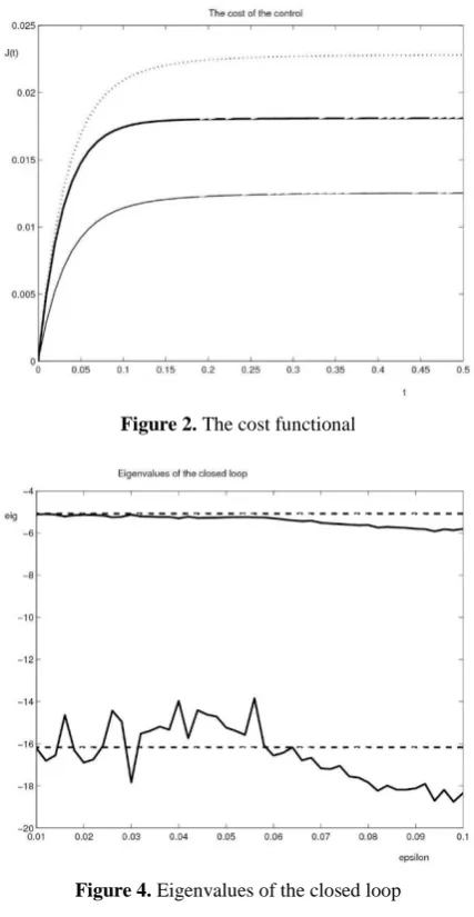
Fig. 2 shows the value of the cost functional. The meaning of the lines (thin / bold) is the same as in the previous figure, moreover, the dotted line shows the cost given by the right-hand side of the inequality (6). This is in some sense a limit cost that cannot be exceeded. This is indeed the case.
Now we investigate the influence of the variable ε ε olution. One can expect that, in case this limit is too tight, the absolute value of the minimized elements (in our case, K1,2) increases. This is since in this case the
decentralized control cannot be found such that the condition (6) is satisfied. Then, the algorithm is forced to yield a centralized controller even if the resulting value of the objective function is high. This effect is illustrated in Fig. 3. Moreover, numerical experiments show that the rapid changes of the value in the left-hand part of the graph are also partially due to high sensitivity of the computational algorithm on the data. The remedy is to use the values ε around which the solution remains more or less constant. This threshold seems to be the value ε=0.06 in our case.
Dependence of the eigenvalue of the closed loop on the variable ε, shown in Fig. 4, is also noteworthy. The dashed lines represent the eigenvalues of the closed loop under the centralized feedback while the solid lines stand for the eigenvalues of the closed loop under decentralized feedback. The part for ε<0.06 should be rather disregarded due to reasons described above.
Example 2: reference tracking
In this case we consider the same system as in the previous example. However, in this case, we require the state x1 to be a constant (defined later) while the
state x2 should track a sine trajectory. Hence the
reference generator is
2. 3 3, 2
1=0,q =q q = q
Figure 1. States of the system
Figure 3. States The entry K12
Figure 5. The tracking error
Figure 2. The cost functional
Figure 4. Eigenvalues of the closed loop
Figure 6. The cost functional
Amplitude and phase are given by initial conditions in this reference generator. Let us define
. 01 . 0 , 0001 . 0
, 0 100 0 100 0
0 0 10 0 10
I R I C
C Q
C
T
Again, the aim is to design a decentralized control such that the performance is not much worse than the performance of the LQ control. In this case we require to minimize the information exchange from xi into uj
This means the objective function is defined as
( ) ( ) 10 ( )2
.2 , 1 6 2
1 , 2 2
2 ,
1 nD nD
nD Y Q
Y
Minimize
The condition (6) was chosen asPD<PC+45I. Then the decentralized control law is given by
. ) (
) ( ) (
, 002 . 0 35 . 1 0 34 . 1 0
0 0 3 . 0 0 3 . 0 103
t q
t x K t u K
Fig. 5 shows the tracking error. Fig. 6 illustrates the cost functional.
6. Conclusions
An algorithm for decomposition of a large system was presented. It is based on solution of a set of LMIs. The algorithm is easy to implement. The results were illustrated using simulations.
Acknowledgments
We would like to present our thanks to anonymous reviewers for their helpful suggestions.
References
[1] M. Singh. Decentralized Control. North-Holland, Amsterdam, 1981.
[2] M. Jamshidi. Large Scale Systems: Modeling, Control and Fuzzy Logic. Prentice Hall, New Jersey, 1997. [3] V. Tsurkov. Hierarchical Optimization and
Mathema-tical Physics. Kluwer, Dordrecht, 2000.
[4] V. Tsurkov. Large Scale Optimization - Problems and Methods. Kluwer, Dordrecht, 2001.
[5] M. Singh, A. Titli. Systems: Decomposition, Optimi-zation and Control. Mashinostroenye, Moscow, 1986 (in Russian).
[6] L. Trave, A. Titli, A. Tarras. Decomposition, Fixed Modes and Structure Constraints. Springer, Berlin,
1989.
[7] D. D. Šiljak. Decentralized Control of Complex Systems. Academic Press, Boston, 1991.
[8] J. Finney, B. Heck. Matrix Scaling for Large-Scale System Decomposition. Automatica, 1996, Vol. 32, No. 8, 1177-1181.
[9] X. B. Chen, S. Stankovic. Decomposition and decentralized control of systems with multi-overlapping structure. Automatica, 2005, Vol. 41, No. 10, 1765-1772.
[10] J. G. Lee, V. G. Vogt, M. H. Mickle. Optimal Decomposition of Large-Scale Networks. IEEE Transactions on Systems, Man, and Cybernetics, 1979, Vol. 9, No. 7, 369-375.
[11] A. S. R. Ferreira, M. Arcak, E. Sontag. A Decomposition-Based Approach to Stability Analysis of Large-Scale Stochastic Systems. In: Proceedings of the American Control Conference, Montréal, Canada, June 27-29, 2012, pp. 6382-6387.
[12] H. S. Shin, S. Lall. Decentralized Control via Gröbner
[13] Bases and Variable Elimination. IEEE Transactions on Automatic Control, Vol. 57, No. 4, 2012, 1030 - 1035. [14] W. Chang, W.-J. Wang, N.-J. Li, H.-G. Chou,
J.-W. Chang. H∞ Control Synthesis for the Large-Scale System Based on a Linear Decomposition of Nonlinear Interconnections. International Journal of Fuzzy Systems, 2014, Vol. 16, No. 1, 97-110.
[15] J. Anderson, Y. C. Chang, A. Papachristodoulou. Model decomposition and reduction tools for large-scale networks in systems biology. Automatica, 2011, Vol. 47, No. 6, 1165-1174.
[16] N. Soranzo, F. Ramezani, G. Iacono, C. Altafini. Decompositions of large-scale biological systems based on dynamical properties. Bioinformatics, Vol. 28, No. 1, 2012, 76-83.
[17] D. Stipanovic, G. Inalhan, R. Teo, C. Tomlin. Decentralized Overlapping Control of a Formation of Unmanned Aerial Vehicles. Automatica, Vol. 40, No. 8, 2004, 1285-1296.
[18] F. Fonteneau-Belmudes, D. Ernst, C. Druet, P. Panciatici, L. Wehenkel. Consequence driven decomposition of large-scale power system security analysis. IREP Symposium – Bulk Power System Dynamics and Control – VIII, Buzios, RJ, Brazil, August 1-6, 2010, 1-8.
[19] D. D. Šiljak, A. I. Zečevic. Control of large-scale systems: Beyond decentralized feedback. Annual Reviews in Control, 2005, Vol. 29, No. 2, 169-179. [20] B. Labibi, H. J. Marquez, T. Chen. LMI
optimiza-tion approach to robust decentralized controller design.
International Journal of Robust and Nonlinear Control, 2011, Vol. 21, No. 8, 904-924.
[21] A. Zemouche, A. Alessandri. A New LMI Condition for Decentralized Observer-Based Control of Linear Systems with Nonlinear Interconnections. In:
Proceedings of the 53rd IEEE Conference on Decision and Control, Los Angeles, California, USA, December 15-17, 2014, pp. 3125-3130.
[22] J. Anderson, A. Papachristodoulou. Dynamical Sys-tem Decomposition for Efficient, Sparse Analysis. In:
Proceedings of the 49th IEEE Conference on Decision and Control, Dec. 15-17, 2010, Atlanta, GA, USA, pp. 6565-6570.
[23] S. Boyd, L. El Ghaoui, E. Feron, V. Balakrishnan. Linear Matrix Inequalities in System and Control Theory. SIAM, Philadelphia, 1994.
[24] S. Stankovic, D. D. Šiljak. Robust stabilization of nonlinear interconnected systems by decentralized dynamic output feedback. Systems & Control Letters,
2009, Vol. 58, No. 4, 271-275.
[25] B. Rehák. Optimization-based Decomposition of a Large-Scale System. In: Proceedings of the IFAC Workshop on Applications of Large Scale Industrial Systems, Helsinki, Finland, August 30-31, 2006, pp. 47-52.
[26] B. Rehák. Decomposition of a Large-Scale System and Reference Tracking: LMI-based Approach. In:
Proceedings of the IFAC conference on Large Scale Systems, Gdansk, Poland, July 23-25, 2007, pp. 374-379.
[27] T. Kailath. Linear Systems, Prentice Hall,Englewood Cliffs, 1980.