Nonlinear Slip Effects on Pipe Flow and Heat Transfer of Third Grade Fluid with Nonlinear Temperature-Dependent Viscosities and Internal Heat Generation

(1)

http://www.sciencepublishinggroup.com/j/se doi: 10.11648/j.se.20180603.11

ISSN: 2376-8029 (Print); ISSN: 2376-8037 (Online)

Nonlinear Slip Effects on Pipe Flow and Heat Transfer of

Third Grade Fluid with Nonlinear Temperature-Dependent

Viscosities and Internal Heat Generation

Gbeminiyi Sobamowo

1

, Akinbowale Akinshilo

1

, Ahmed Yinusa

1

, Oluwatoyin Adedibu

2

1_{Department of Mechanical Engineering, University of Lagos, Yaba, Nigeria} 2

Department of Electrical Engineering, the Polytechnic, Ibadan, Nigeria

Email address:

To cite this article:

Gbeminiyi Sobamowo, Akinbowale Akinshilo, Ahmed Yinusa, Oluwatoyin Adedibu. Nonlinear Slip Effects on Pipe Flow and Heat Transfer of Third Grade Fluid with Nonlinear Temperature-Dependent Viscosities and Internal Heat Generation. Software Engineering.

Vol. 6, No. 3, 2018, pp. 69-88. doi: 10.11648/j.se.20180603.11

Received: July 8, 2018; Accepted: July 19, 2018; Published: August 21, 2018

Abstract:

The various industrial, biological and engineering applications of third grade fluid have in recent times propel continuous research on the flow dynamics and heat transfer characteristics of the non-Newtonian fluid. In this work, effects of nonlinear hydrodynamic slip and temperature-jump conditions on pipe flow and heat transfer of third grade fluid with nonlinear temperature-dependent viscosities and internal heat generation are presented. The developed nonlinear governing equations are solved using regular perturbation method. In order to verify the accuracy of the solution methodology, the results of the approximate analytical solution are compared with the results of the numerical solutions using Runge-Kutta fourth-order coupled with shooting method. Good agreements are obtained between the analytical and the numerical results. Thereafter, the obtained approximate analytical solutions are used to investigate the effects of variable viscosity, non-Newtonian parameter, viscous dissipation and pressure gradient on the flow and heat transfer characteristics of the third-grade fluid in the pipe under Reynolds’s and Vogel’s temperature-dependent viscosities. The present results can be used to advance the analysis and study of the behaviour of third grade fluid flow and steady state heat transfer processes such as found in coal slurries, polymer solutions, textiles, ceramics, catalytic reactors, oil recovery applications etc.

Keywords:

Third-Grade Fluid, Pipe Flow, Non-Linear Viscosities, Non-Linear Internal Heat Generation, Nonlinear Boundary Conditions

1. Introduction

The generalization of Navier–Stokes’ model to highly non-linear models of non-Newtonian fluids has received considerable attention in the past few decades. One of the earliest classes of such models is the differential type model of which the third grade fluid is one of the most popular subclasses of the differential type fluids. The third grade fluid is a non-Newtonian fluid which its viscosity varies based on the applied force. It is a favored fluid due to the exciting phenomena it captures such as the shear thinning and thickening effects. The mathematical model of the third grade fluid represents a more realistic description of the behavior of non-Newtonian fluids. The model also represents a further attempt towards the study of the flow structure of

(2)

improve the characteristics of the visco-elastic properties of the fluid, the stability of the third grade fluid model was studied by Fosdick and Rajagopal [1] while Majhi and Nair [2] investigated the effects of stenotic geometry and the non-Newtonian parameter of the third grade fluid on the resistive impedance and wall shearing stress. Their results were compared with similar study submitted by Massoudi and Christie [3] who presented the numerical solutions on the effects of variable viscosity and viscous dissipation on the flow of third grade fluid in a pipe using the finite difference method. Yurusoy and Pakdemirli [4] developed approximate analytical solution for the flow of the third grade fluid in a pipe using constant viscosity model, variable viscosity models under no slip condition while Vajrevelu et al [5] presented a numerical solution for the third grade fluid flows between rotating cylinder using Schauder theory and perturbation technique. The fluctuating behaviour of magnetohydrodynamic rotational flow of the third grade fluid on a porous plate was studied by Hayat et al. [6]. The similarity solutions to boundary layer equation for the third grade fluid were developed by Muhammet [7] using the special coordinate system generated by the potential flow. The steady flow analysis of the third grade fluid between circular concentric cylinders with heat transfer was presented by Yurusoy [8]. In the study, the pipe temperature is assumed to be higher than fluid temperature. Also, Pakdemirli and Yilbas [9] developed approximate analytical solution of non-Newtonian fluid using Vogels viscosity model and entropy generation in a pipe. The steady flow of a third grade fluid past a porous horizontal plate with partial slip was investigated by Sajid et al. [10]. Elahi et al. [11] used implicit finite difference method to analyze the unsteady free convective flow of a third grade fluid past an infinite vertical plate when uniform suction is applied at the plate. Jayeoba et al. [12] presented the analytical approximate solution to determine the temperature fields for steady flow of a third grade fluid in a pipe with models of viscosities including a heat generation term for the no slip boundary condition. Most of the studies previously carried out on the third grade fluid are limited to no slip flow condition which is a simplified method of predicting the actual behavior of the fluid in various applications. In practice most problem of fluid flow exists as either partial slip or slip condition. Therefore, Ogunmola et al. [13] presented perturbation solutions for the non-linear analysis of the flow of third grade fluid with temperature-dependent viscosities and internal heat generation. In their work, a linear variation of source term with temperature was assumed and the non-linear slip boundary conditions were linearized. Abbasbandy et al. [14] and Nayak et al. [15] presented numerical results for the flow of third grade fluid between two porous walls, and porous vertical plate, respectively. Aiyesimi et al. [16] analyzed the

unsteady magnetohydrodynamic thin flow of a third grade fluid with heat transfer and under no slip condition in an inclined plane. Effects of variable viscosity on the flow of a third grade fluid flowing over a radiative surface with Arhenius equation was studied by Ogunsola and Peter [17] while Yunusoy et al. [18] obtain the perturbation solution for the analysis of the flow of third grade fluid flow between two parallel plates. Moreover, different approximate analytical methods have been used to analyze the flow of fluid in pipe, channels and over a plate under the influences of hydrodynamic slip boundary conditions [19-27]. In this work, regular perturbation method is used to develop approximate analytical solutions for the non-linear models for the pipe flow of third grade fluid with temperature-dependent viscosities and internal heat generation under third-degree non-linear hydrodynamic slip and temperature-jump conditions are presented. Effects of non-linear variations of internal heat generations with temperature are studied under Reynold and Vogel’s temperature-dependent viscosities. Also, the develop models were used to investigate the effects of other flow parameters on the flow behaviour and heat transfer characteristics of the third grade fluid.

2. Problem Formulation

The Cauchy stress tensor for an incompressible homogeneous thermodynamically compatible third grade fluid is given by

T= - I +µ + + + S (1)

where

S = + ( + ) + ( )

T is the stress tensor, is the pressure, I is the identity

tensor, µ is the dynamic viscosity and (I =1, 2), (1, 2, 3) are material constants.

= ( ) + ( )T

=_!"!A + ( ) + ( )T

A1

Generally, the _$ areRivlin- Ericken tensor defined as

%=_{!" %&}! + %& L+ '( %& ; for n>1 (2)

where V denotes velocity field, grad is the operator gradient and d/dt is the material time derivative. When the motions of the fluid are thermodynamically compatible, the Clausius-Duhem inequality and the assumption that the Helmholtz free energy is minimum when the fluid is locally at rest require that

= = 0, ≥ 0, µ≥ 0, ≥ 0 [ + ] ≤ √24/ (3)

Since > 0 the stress tensor can predict shear thickening as well as the normal stress. Thus stress tensor relation can be written as

(3)

Where velocity field can be expressed as

V=v (r) (5)

And temperature field as

θ = θ (r) (6)

substituting velocity field using the modified constitutive relation in the balance of linear momentum in the absence of body forces and assuming fluid can only undergo isochoric motion (i.e. div v=0), we have a partial differential equation of the form

12

1" = div T + b (7)

Consider the flow of a third grade fluid in an infinitely long pipe as shown in Figure 1. The momentum and temperature equation with incorporated quadratically varying source term with temperature are given by system of differential Eqs. (8, 9, 10, 11)

3 !

!34 (2 ∝ ∝ 6

!7 !38 9

1:

13 (8)

0 1:_1∅ (9)

3 ! !3< /

!7 !3= 3

!

!342 6

!7 !38 9

1:

1> (10)

? 4₃_!3! < !(_!3=9 / <!7_!3= 2 <!7_!3=@ ABC D E DF 0 (11)

Figure 1. Physical model and coordinate system.

The slip condition at the pipe wall can be introduced in terms of shear stress. In their paper, ogunmola et al. [13] used linearized forms of hydrodynamic slip and temperature-jump conditions (first-order boundary conditions) given in Eq. (12) to analyze the flow problem.

G H I 6!7_!38J_3KL, M D H E DN E? 6!(_!38J_3KL (12)

In this work, non-linear hydrodynamic slip and temperature-jump conditions (third- and fourth-order boundary conditions) given in Eq. (13) are applied.

G H I O!7_!3 PQ R <

!7

!3= ST_3KL, M D H E DN E? O !( !3 / <

!7

!3= 2 < !7

!3= @

ST

3KL (13)

At the center of the pipe, the boundary condition is given as

!7

!3 0 0,

!(

!3 0 0 (14)

using the dimensionless parameters as stated in the nomenclature, the dimensionless equation (leaving out the bars on the equations for conveniences) for Equs. (10 and 11) yields the following:

!R !3

!7 !3

R 3<

!7 !3

3!U₇

!3U= V₃<!7_!3= <!W_!3 3! U₇

!3U = B (15)

!U_X

(4)

And the dimensionless boundary conditions under slip condition are given as

G H ] O!7_!3

Λ

<!7_!3= ST

3KL, \ = −^ O !X !3+

Γ

/ <

!7

!3= +

ΓΛ

< !7 !3=

@

ST

3KL (17)

G_{(0) = 0,} \_{(0) = 0}

where

D = 1+ 8Kn and Ap = -2Kn

In this work, two equations of temperature-dependent viscosity, namely, the Reynolds and the Vogel’s models are used.

i. Temperature-dependent viscosity using Reynolds model

/(D) = /F_`&a((&(b)c (18)

ii. Temperature-dependent viscosity using Vogel’s model

/(D) = /F_`d/(f&(b)c (19)

The non-dimensionalized form of the temperature-dependent viscosity using Reynold’s and Vogel’s model are

/ = _(−g\) (20)

/ = _(h/(^&X)&(b)₍₂₁₎

2.1. Analysis of the Flow Heat Transfer in the Pipe Using Reynold’s Model of Viscosity

The regular perturbation technique is used to determine the approximate analytical solution for the Reynold’s viscosity model.

Taking the Maclaurin’s series, Eq. (20) takes the form

/ = _ij(−g\) = 1 − g\ + l(g ) (22) Series solutions of the equation of the velocity and

temperature may be obtained by using perturbation method taking m as the perturbation parameter. Solutions are obtained in the form.

G = GF+ mG + l(m ) (23)

\ = \F+ m\ + l(m ) (24)

Substitute Equ. (23 and 24) into Equ. (14) and changing parameters in the terms yields.

Where Λ = mn, [ = mo, I = mp

l(mF_): !U7b

!3U + !7_!3b= B (25)

l(m ): G + G − p\F GF− p\F GF− p GF \F

= −n <!7b

!3= < !7b

!3 + 3 !U₇_b

!3U= + B (26) Also, substitute Equ. (23), 24 and 26) into Equ. (15) and changing parameters in the terms yields

l(mF_): !UXb

!3U + !X_!3b+!X_!3b+ Γ <!7_!3b= = 0 (27)

\(m ): !UXs

!3U + !X_!3b+!X_!3s+ Γ <!7_!3b= . 4n <!7_!3b= −

p\F9 + 2Γ !7_!3b!7_!3s+ o\C = 0

(28)

The boundary conditions for the leading order equation are

!7b

!3 (0) = !Xb

!3 (0) = 0 (29)

GF(H) = ] O!7_!3b+

Λ

<!7_!3b= ST

3K_us, \F= −^ O !Xb

!3 +

Γ

/ < !7b

!3= +

ΓΛ

< !7b

!3= @

ST

3K_us (30)

With the boundary conditions it could be easily shown that Eq. (29) gives

GF=v_@6 +_xw+Vv

U_w

xQ −_xU8 (31) and

\F= −yv

U₃z

{@ + yvU

{^ xQ− yv U

@^ xU− Vyv z

{^ xz+ yv U

{@xU (32) Also, for the first-order equation, the boundary conditions are given as

!7s

!3 (0) = !Xs

!3 (0) = 0 (33)

G (H) = ] O!7s

!3 + Λ < !7s

!3= ST_3Ks u

, \ = −_^ O!Xs

!3 + Γ/ < !7s

!3= + ΓΛ < !7s

!3= @

ST

3K_us (34)

where

(5)

Substituting the corresponding terms from the solutions in Equs. (31) and (32) into Equ. (26) and (28) and integrate twice subject to the boundary condition in Equ. (33) and (34) yields.

G E|yU_{@}Q~• |y}_{@xQ~QUE|€y} Q_~U {xU E|€y}

•_~U

{@xz |y}

Q_~U ‚{xz E|y}

Q_~•

‚ E

avQ3z

ƒ E

w|yUvQ ƒ@x• w|yv

Q

xz Ew|„yv Q

ƒxQ Ew|„yv • x• w|yv

Q ƒx•E w|yvQ

… x•Ewav • xQ E wav

Q xQ w†yv

Q

xz w†„yv Q

ƒxQ w†„Vyv

• x• Ew†yv

Q

ƒx• ] 6†|v •_y• @‚‡{xˆ †|v

•_yU F@ƒx‰E†|„v

•_yU ‚ xŠ E†|„v

Š_yU F@ƒxˆ E†|v

•_yU ƒ … xˆE †|v

•_yU ƒƒxˆE †ya}•

F@ƒxŠE †ya} • F@ƒxŠ †|„y

Q_}• { @@x‰ E†‹€y

U_}•

‚ xŠ †‹€

U_yU_}• ƒx• †‹€

U_yU_}Š ‚ x‰ E†‹€y

U_}• F@ƒxŠ †‹€y

U_}•

F‡ x‰ †Œ€y} •

‚ x• †€yŒ}

• ‚ x• E †‹€y

U_}• ‚ {xŠ †‹€yU}•

ƒx• E†‹€ U_yU_}•

x• E †‹€ U_yU_}Š ƒxŠ †‹€y

U_}• ‚ x• E †‹€y

U_}•

‡{ƒxŠ E†Œ€y} •

ƒx• E †Œ€y} •

ƒx• E†‹€Vy Q_}Š

{ @@xˆ †‹€Vy U_}Š ‚ xŠ E †‹€

U_VyU_}z ƒxŠ E†‹€

U_VyU_}ˆ ‚ xˆ †‹€VyU}Š

F@ƒxˆ E†‹€y U_}Š

F‡ xˆ E†Œ€Vy} Š

‚ xŠ E †Œ€Vy} Š ‚ xŠ †‹y

U_}• @‚‡{xˆE†‹y

U_}• F@ƒx‰ †‹€y

U_}• ‚ xŠ †‹€y

U_}Š F@ƒxˆ E†‹y

U_}• ƒ … xˆ †‹y

U_}• F@ƒx‰ E †‹y

U_}•

ƒƒxˆ †yav • F@ƒxŠ †yav•

F@ƒxŠ8 |y U_}U F@x•E|yv

Q {@x• |„yv

Q {xz |„yv

• {@x• E |yv

Q ‚{x• |yv

Q

‚ x• av Q

ƒxz av Q

ƒxz (35)

Substitute Equs. (31 and 34) into Eq. (26) and then changing the terms back to original parameters, finally gives

w v_@6 _xw Vv_x_QUwE_x_U8 E|yU_{@}Q~• |y}_{@xQ~_QUE|€y}_{xQ_U~UE|€y}_{@x•_z~U |y}_‚{xQ~_zUE|y}_‚Q~•EavQ_ƒ3zEw|y_ƒ@xUv_•Q w|yv_x_zQEw|„yv_ƒx_QQE

w|„yv• x• w|yv

Q ƒx•E w|yv

Q … x•Ewav

• xQ E wav

Q xQ w†yv

Q

xz w†„yv Q

ƒxQ w†„Vyv

• x• Ew†yv

Q

ƒx• ] 6†|v •_y• @‚‡{xˆ †|v

•_yU F@ƒx‰E†|„v

•_yU ‚ xŠ E†|„v

Š_yU F@ƒxˆ E †|v•_yU

ƒ … xˆE †|v •_yU

ƒƒxˆE†ya} •

F@ƒxŠE †ya} • F@ƒxŠ †|„y

Q_}• { @@x‰ E†‹€y

U_}•

‚ xŠ †‹€

U_yU_}• ƒx• †‹€

U_yU_}Š ‚ x‰ E†‹€y

U_}• F@ƒxŠ †‹€y

U_}•

F‡ x‰ †Œ€y} •

‚ x• †€yŒ}

• ‚ x• E †‹€yU_}•

‚ {xŠ †‹€y U_}• ƒx• E†‹€

U_yU_}• x• E †‹€

U_yU_}Š ƒxŠ †‹€y

U_}• ‚ x• E †‹€y

U_}•

‡{ƒxŠ E†Œ€y} •

ƒx• E †Œ€y} •

ƒx• E†‹€Vy Q_}Š

{ @@xˆ †‹€Vy U_}Š ‚ xŠ E †‹€

U_VyU_}z ƒxŠ E †‹€U_VyU_}ˆ

‚ xˆ †‹€Vy

U_}Š F@ƒxˆ E†‹€y

U_}Š

F‡ xˆ E†Œ€Vy} Š

‚ xŠ E †Œ€Vy} Š ‚ xŠ †‹y

U_}• @‚‡{xˆE†‹y

U_}• F@ƒx‰ †‹€y

U_}• ‚ xŠ †‹€y

U_}Š F@ƒxˆ E†‹y

U_}• ƒ … xˆ †‹y

U_}• F@ƒx‰ E †‹yU}•

ƒƒxˆ †yav •

F@ƒxŠ †yav • F@ƒxŠ8 |y

U_}U F@x•E|yv

Q {@x• |„yv

Q {xz |„yv

• {@x• E |yv

Q ‚{x• |yv

Q ‚ x• av

Q

ƒxz av Q

ƒxz (36)

Following the same procedural approach, we have for the dimensionless temperature as

\

E

ΓB₆₄2 4

+

ΓB2

16Ž••3

−

ΓB

2

4Ž••2

−

ΛΓB

4

16Ž••4

+

ΓB

2

64•2

+

ayU_vz₃•

‚‡{ + |yU_vz₃‰

{ ƒ@ - |yU_vz₃z

F @^ xQ+ |y

U_vz₃z

‚{^ xU +|yVv

•₃z

F @xz − |y

U_vz₃z

@F…{xz −

|yQvz3‰ @‚‡{ +

|yUvz3z ‚ xQ − |y

U_vz₃z

ƒ^ xU −|y

U_v•₃z

‚ ^ xz +|y

U_vz₃z

F@ƒxz −|y

U_vz₃‰

ƒƒ − yavz3•

‚ − yavz3•

‚ − ‘yvU3•

F@ + ‘yvU3• {@^ xQ -‘yv

U₃U

{^ xU−‘Vyv

z₃U

{@^ xz +

‘yvU3U ‚{xz −yŒv

U₃U

‚{^ xz− yŒv z

…{^ x•− |y

U_vz

F@ƒ^ xŠ+ |y

U_vz

‚{^U_x•− |y

U_vz

{@^U_x•− |Vyv •

‚{^U_xŠ+ |y

U_vz

F @^ xŠ + |y

Q_vz

F‡ ^ xŠ − |y

U_vz

ƒ^U_x•+ |y

U_vz

^U_x•+

|yUv• ƒ^U_xŠ |y

U_vz

‚ ^ xŠ+ |y

U_vz

‚ {^ xŠ+ yav z

… ^ x• + yav z

… ^ x• + ‘yv U

ƒ@^ x•− ‘yv U

^U_xz+ ‘yv U

ƒxQ_^U+ ‘yVv z

x•_^U+ ‘yv U

^ x•− ‘yv U

ƒ^ x• − |y

Q_vz

ƒ@^ x• +

|yUvz ^ x• − |y

U_}z

ƒ^U_xz − |y

U_v•

^U_x•+ |y

U_vz

ƒ^ x• − |y

U_vz

… ^ x• − yav z

^ xz− yav z

^ xz− ‹†y

z_v•

@‚‡{^ xsb+ ‹†y

Q_v•

F@ƒ^ xsb− ‹†y

Q_v•

‚‡ ^U_x‰− ‹†y

Q_v‰

F@ƒ^U_xsb+

‹†yQv•

ƒ … ^ xsb− ‹†y

Q_v•

ƒƒ^ xsb− Œ†y

U_v•

F@ƒ^ x‰− Œ†y

U_v•

F@ƒ^ x‰+‹„

U_†yz_v•

{ @@xˆ − ‹†y

Q_v•

‚ ^U_x‰+ ‹†y

Q_v•

ƒ^Q_xŠ+ ‹†y

z_v‰

‚ ^Q_xˆ− ‹†y

Q_v•

F@ƒ^U_xˆ+ ‹†y

Q_v•

F‡ ^U_xˆ+ Œ†y

U_v•

‚ ^U_xŠ+

Œ†yU_v•

‚ ^U_xŠ - ‹†y

z_v•

‚ {^U_x‰+ ‹†y

Q_v•

ƒ^U_xŠ− ‹†y

Q_v•

^Q_x‰− ‹†y

Q_v‰

ƒ^Q_x‰+ ‹†y

Q_v•

‚ ^U_x‰− ‹†y

Q_v•

‡{ƒ^U_x‰− †y

U_v•_a

ƒ^U_x•− †y

U_v•_a

ƒ^U_x•− |†y

z_v‰_V

{ @@^U_xsb+|†y

Q_v‰_V

‚ ^U_xˆ -

|†yQ_v‰_V

ƒ^Q_x• +|†y

Q_vsb_V

‚ ^Q_xsb+ |†y

Q_v‰_V

F@ƒ^U_xsb − |†y

Q_v‰_V

F‡ ^U_xsb−a†y

U_v‰_V

‚ ^U_x‰ - a†y

U_v‰_V

‚ ^U_x‰ + |†y

z_v•

@‚‡{^ xsb− |†y

Q_v•

F@ƒ^ xˆ+ |†y

Q_v•

‚ ^U_x‰+ |†y

Q_v‰

F@ƒ^U_xsb−

|yQ_v•

ƒ … ^ x•+ |’y

Q_v•

ƒƒ^ xsb+ ay

U_v•_†

F@ƒ^ x‰− ay

U_v•_†

F@ƒ^ x‰− |y

Q_Vv•

‚ {^ x‰+ |y

U_v•_V

ƒ^ xŠ - |y

U_v•_V

^U_x• - |y

U_v‰_V

ƒ^U_x‰+|y

U_v•_V

‚ x‰ −|y

U_v•_V

‡{ƒ^ x‰− ayv

•_V

ƒ^ x•− ayv

•_V

ƒ^ x•−

ayvz

‚ {x•− |y

U_vz

{ ƒ@x‰+ |y

U_vz

F @^ xŠ− |y

U_vz

‚{^ x•− |y

U_vz

F @^ x‰+ |y

U_vz

@F…{x‰ + |y

Q_vz

@‚‡{x‰−|y

U_vz

‚ xŠ+ |y

U_vz

ƒ^ x•+ |y

U_v•

‚ ^ x‰− |y

U_v•

‚ ^ x‰− |y

U_vz

F@ƒx‰ +

|yU_vz

ƒƒx‰+ ayv z

‚ x• + ayv z

‚ x•+ ‘yv U

F@x•− ‘yv U

{@^ x•+ ‘yv U

{^ xz + ‘Vyv z

{@^ x•− ‘yv U

F@x•− ‘yv U

‚{x• (37) We can change M, N and P in the above to the terms in the governing dimensionless equations since Λ = mn, [ = mo, I =

mp.

2.2. Analysis of the Flow Heat Transfer in the Pipe Using Vogel’s Model of Viscosity

With the aid of Maclaurin series, the Vogel’s viscosity model can be written as

/ = _ij <h_^− DF= 41 −“hX_^U + l(m )9 = _ij <h_^− DF= <1 −“hX_^U= (38)

Taking the series solution of the velocity and temperature fields yields the expansion

G = G + mG + l(m ) (39)

(6)

Substitute Equ. (38, 39 and 40) into Equ. (14) and change parameters in the terms yields.

l mF _: !U7b

!3U !7_!3b B (41)

l m :!7s !3

!U₇_s

!3U E p\F!7_!3bE p\F! U₇_b

!3U E p !7_!3b!X_!3b En <!7_!3b= <!7_!3b 3 ! U₇_b

!3U= B (42)

Also, substitute Equ. (38, 39 and 40) into Equ. (15) and change parameters in the terms yields.

l mF _: !UXb

!3U !X_!3b !X_!3b Γ <!7_!3b= = 0 (43) \(m ): !UXs

!3U + !X_!3b+!X_!3s+ Γ <!7_!3b= . 4n <!7_!3b= − p\F9 + 2Γ !7_!3b!7_!3s+ o\C = 0 (44)

Following the same procedural analysis as carried out previously subject to the same boundary conditions, we have the dimensionless velocity for the Vogel’s Model of Viscosity as

w=_@6B∗ + wv3_x + wVv_x_Q∗Q−_xv∗_U8 +_^h_U6&yvv_F@∗U3•−„yvv_{@x∗_Q3U+„Vyv_ƒx∗Q_U3U+„yv_@xv∗U3U−yvv_‚{x∗3_zU8 -hyvv_ƒFF^∗3_U•−Vv∗z_v3z+hw_^_U6&yv_ƒ@xUv∗_Š3•−

„yvUv∗

xz +„Vy}v ∗Q

@xQ +„yv ∗

xU −yv

U_v∗U

ƒx•8 − hwyv U

{Fxz_^U−Vwv ∗Q

ƒxQ + _@^VwhU _^hU6&yvv ∗z

ƒ@xŠ −„yvv ∗z

x• +„Vyv ∗•

@x• +„yv ∗z

@xz_v−yvv ∗z

ƒxŠ8 − hwVyvv ∗Q

{F@^U_x• −

VU_•}∗•

vx• −_^hU_^hU6&yvv ∗U

F@x•−„yvv ∗

{@x• +„Vyv ∗Q

ƒxz +„yv ∗U

@xU_v − yvv ∗

‚{x•8+ hyvv ∗

ƒFF^U_x• +Vv ∗z

vxz (45) The dimensionless temperature for the Vogel’s Model of Viscosity is given as

\ =&–vv_{@∗3z−&„–vv_{xQ∗+„V–v ∗U

xU +„–v ∗

vx − –vv∗

{@xz+–vv

∗_h

@^U 6&–vv

∗₃‰

@F…{ − –vv∗₃z

‚^ xQ+V–v

∗U₃z

^ xU + –v

∗₃z

{vx^ − –vv∗₃z

F @xz8 −h–_^UO4&–v

U_v∗U₃‰

@F…{ − –vU_v∗U₃z

‚ +

V–vv∗Q₃z

… ^ xU +–v

∗U₃z

x^ −

–vU_v∗U₃z

F@ƒxz 9 −h–v

U_v∗₃Š

^U_‡ƒ@F −avv

∗z₃•

ƒƒv S − –av∗z₃•

‚‡v + –‘vv∗₃•

F@ + –‘vv∗₃U

{@^ xQ −V–v

∗_‘3U

ƒ^ x − –v∗₃U_‘

@^ vx + –vv∗_yU_‘

‚{xz −–vv

∗_h

@^ ^U6−–vv ∗

‚ xQ− –vv ∗

{@^ x•+V–vv ∗U

ƒ^ x• + –v ∗

@^ vxz− –vv ∗

‚{xŠ8 +h–_^UO4&–v

U_v∗U

‚ ^ xŠ −–v

U_v∗U

ƒxQ +V–vv ∗Q

^U_x•+ –vv ∗U

ƒ^U_vxz−–v

U_v∗U

‚ xŠ9 −

h–vUv∗

‡ F^U_^U_x•− avv ∗z

@ƒvx•_^US + –av ∗z

…{^U_x•− –‘vv ∗

ƒ@^ x•−–‘vv ∗

^ xz+V–‘v ∗U

@^U_xU + –‘v ∗

v^U_xU− –‘vv ∗

ƒ^ x•+h

U_yV–vU_v∗•

ƒ‚ƒF^U_xsU+h

U_yV–vU_v∗•

…ƒ‚{^ ^z_x‰−h

U_yVU_–U_v∗Š

^ ^z_xˆ−

hU_yV–U_v∗•

{ {^ ^U_xˆ + h

U_–U_yVvU_v∗•

…@ @^z_x‰ +h

U_yV–U_vU_v∗•

‚ƒ‚ F^U_xss+hyV–av ∗‰

@{@^U_xsb+h

U_yV–U_vU_v∗•

…ƒ‚{^ ^U_xss+‚h

U_yV–U_vU_v∗•

@F…{^U_^U_xsU - ‚h

U_VU_y–U_vv∗Š

‚ ^U_^U_xˆ -‚h

U_yV–U_v∗•

‚{^U_^U_xz+‚h

U_yV–U_vU_v∗•

{ ƒ@^ ^U_xss+

hU_yV–U_vU_v∗•

@F…{^ xss +‚hyV–

U_vU_v∗‰

F @^ ^U_xˆ −h

U_yVU_–U_vv∗Š

@‡ ^ ^U_xss−‚h

U_yVU_–U_vv∗Š

F @^U_^U_xˆ +‚h

U_yVQ_–U_v∗•

{@^U_^U_x• +‚h

U_yVU_–U_v∗Š

^U_^z_xŠ_v −‚h

U_yVU_–U_vv∗Š

F@ƒ^ ^U_xsb −h

U_yVU_–U_vv∗•

‚ ^ ^z_x• −

‚ha–yVUv∗ˆ ƒ^ ^U_vx‰ -h

U_yVU_–U_v∗•

{ {^ ^U_xˆ −‚h

U_yV–U_v∗•

‚{^ ^U_x‰ +‚h

U_yVU_–U_v∗Š

^U_^U_vxŠ − ‚yV–

U_v∗•

{^U_^z_x‰_vU−‚yVh

U_–U_v∗•

F @^ ^U_xˆ−h

U_yV–U_v∗•

‚{^ ^U_xˆ−‚hy—ŒVv ∗‰

{@^ ^U_xˆ_vU+h

U_yV–U_vU_v∗•

…@ @^U_xsU +

‚hUyV–UvUv∗• { ƒ@^ ^z_xss−‚h

U_yVU_–U_vv∗Š

F@ƒ^ ^z_xsb −‚h

U_yV–U_v∗•

F @^ ^U_xˆ +‚h

U_yV–U_vv∗z

{‚‚ {^z_xsU +h

U_Vy–U_vv∗•

{ ƒ@^U_xŠ +‚hyV—Œvv ∗‰

@F…{^ ^U_xsb +h

U_Vy–U_vU_v∗•

‚ƒ‚ F^z_xss +h

U_yV–U_vU_v∗•

@F…{^ ^U_xss- h

U_–U_VU_yvv∗•

‚ ^ ^z_xˆ −

hU–UVyv∗• ‚{^ ^U_x‰+h

U_–U_VyvU_v∗•

{ ƒ@^U_xss +h

U_–U_yVvU_v∗z

F@ƒF^z_xsb +h–yVŒv ∗Š

F @xˆ +h–yVŒv ∗•

@{@^U_xsb+‚h–yVŒv ∗‰

F @^U_{^ x}ˆ−‚h–yV

U_Œv∗ˆ

ƒ^U_{v^ x}‰ −‚h–yVŒv ∗‰

{@^U_{^ x}Š_vU+‚h–yVŒv ∗‰

@F…{^U_xsb +

h–yVŒv∗Š

F @^U_xˆ +‚yVŒv ∗sb

‚{vU_x‰ + h

U_–U_vQ_yv∗Q

@ƒ ‚^z_xsb+ h

U_–U_vQ_yv∗Q

F^ ^z_xsb−h

U_–U_vU_yVv∗z

‚@F^ ^z_x‰ −h

U_–U_vU_yv∗Q

‡‡Fv^z_xŠ + h

U_y–vQ_v∗Q

^z_{@… ƒFx}sb+h

U_y–vQ_v∗U

^z_{‡ ‚Fx}ˆ+˜y–av

U_v∗Š

^U _FƒFxsb+

hUy–UvQv∗Q ^U _Fxˆ_^ + h

U_y–U_vQ_v∗Q

^z _{F @x}‰_^U−˜y–

U_vU_v∗z_V

^U _ƒxˆ_^U −h

U_y–U_vv∗Q

^U_{@x•_^U+ h

U_y–U_vQ

^z_@F…{xˆ_^ +h

U_y–U_vQ_v∗U

^z_{‚ F^ x}‰+ ˜y–

U_vv∗•

^U _‚{xŠ_^ −h

U_yV–U_vU_v∗z

^U _ƒ@Fxˆ_^ −h

U_yV–U_vU_v∗z

^U _‚{xŠ_^U +

hUyVU–Uvv∗U ^U _{xz_^U +h

U_yV–U_v∗z

^z_ƒx•_^U −h

U_y–U_vU_v∗Q

^z_{@Fx•_^ −hyŒV—v ∗•

^U _{^ x}• − h

U_y–U_v∗U

^U_‡‡Fx•_^ − h

U_y–U_vv∗Q

^U_{@Fx‰_^U+h

U_y–U_Vv∗z

^U_ƒx•_^U +h

U_y–U_v∗Q

^z_@vxz − hy–

U_vv∗Q

^U _‚{xŠ_^ −h

U_y–U_vv∗U

^U _Fx•_^ −

hy—Œv∗• ^U _{x•_v^ +h

U_y–U_vQ_v∗Q

^U_@F…{xˆ −h

U_yV–U_vU_v∗z

‚ ^ x‰ −h

U_y–U_vv∗Q

^U _‚{xŠ_^ +yh

U_–U_vU_v∗

{ ƒ@^z_xˆ+yh

U_–U_vQ_v∗U

F@ƒF^U_x• +yha–vv ∗•

F @^U_x‰+yh

U_–U_vQ_v∗U

‡ ‚F^U_xˆ +yh

U_–U_vQ_v∗U

‚ F^U_x‰ −

yhU_–U_VvU_v∗Q

{@F^z_xŠ −yh

U_–U_vU_v∗U

F^U_x• +yh

U_–U_vQ_v∗U

F@ƒF^U_xˆ +yh

U_–U_vQ_v∗

‚{FF^z_x‰+yh–avv ∗z

ƒ^U_xŠ +yh–avv ∗Q

FƒF^U_x‰ +y˜a–vv ∗•

‚{^U_{^ x}z−yhV–av ∗•

^U_x•_^ −y—Œ˜v ∗•

{^U_x• + yh–av ∗•

F @^U_x‰+

yhaU_vv∗z

@F^U_x‰+yha

U_vv∗z

ƒF^U_xŠ+ya

U_v∗Š

{@xŠ −–vv

∗_h

@^ 6 &–v∗_v

@F…{x‰− –v

∗_v

‚{^ xŠ+&–Vv ∗U

x• + &–v ∗

{^ x•− –v

∗_v

F @x‰8+h–_^U6<&–v

U_v∗U

@F…{x‰ − –v

U_v∗U

‚ ^ xz+V–vv ∗Q

… x• +

–v∗U

x•−–v

U_v∗U

F@ƒx‰= − h–v

U_v∗

ƒ@F^U_xŠ− av ∗z

ƒƒx•8 +–av ∗z

‚‡{x• −–‘vv ∗

F@x•−–‘vv ∗

{@^ x•+–‘Vv ∗

ƒxQ + –‘v ∗

@vxQ−–‘vv ∗

‚{x• (46)

3. Results and Discussion

(7)

Figure 2. Effect of pressure gradient parameter C on the velocity distribution of Reynolds viscosity model when for Λ = δ = C =γ=1.

Figure 3. Effect of varying parameter Γ on the velocity distribution of Reynolds viscosity model when for Λ = δ = C =γ=1.

Figure 4. Effect of pressure gradient parameter Λ on the velocity distribution of Reynolds viscosity model when γ= Γ = Λ = δ =C= γ= 1.

0 0.05 0.1 0.15 0.2 0.25

-1 -0.8 -0.6 -0.4 -0.2 0 0.2 0.4 0.6 0.8 1

w

r

C =-0.5

C =-0.75

C =-1

0 0.05 0.1 0.15 0.2 0.25

-1 -0.8 -0.6 -0.4 -0.2 0 0.2 0.4 0.6 0.8 1

w

r

Γ =1 Γ =3 Γ =5

0 0.05 0.1 0.15 0.2 0.25

-1 -0.8 -0.6 -0.4 -0.2 0 0.2 0.4 0.6 0.8 1

w

r

(8)

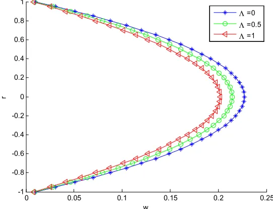
Figure 5. Effect of varying parameter γ for the velocity distribution of Reynolds viscosity model when for Λ = δ = C =Γ =1.

Figure 6. Effect of pressure gradient parameter A on the velocity distribution of Reynolds viscosity model when γ= Γ = Λ = δ = γ=C= 1.

Figure 7. Effect of varying parameter B on the velocity distribution of Reynolds viscosity model when for Λ = δ = C =γ=Γ =1.

0 0.05 0.1 0.15 0.2 0.25

-1 -0.8 -0.6 -0.4 -0.2 0 0.2 0.4 0.6 0.8 1

w

r

γ =-4 γ =0 γ =4

0 0.05 0.1 0.15 0.2 0.25 0.3 0.35

-1 -0.8 -0.6 -0.4 -0.2 0 0.2 0.4 0.6 0.8 1

w

r

A =2 A =1.5 A =1

0 0.05 0.1 0.15 0.2 0.25 0.3 0.35

-1 -0.8 -0.6 -0.4 -0.2 0 0.2 0.4 0.6 0.8 1

w

r

(9)

Figure 8. Effect of pressure gradient parameter C on the velocity distribution of Reynolds viscosity model when γ= Γ = Λ = δ = γ= 1.

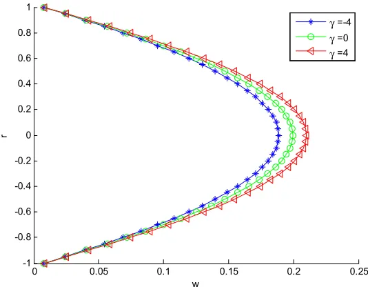
Figure 9. Effect of varying parameter Γ on the velocity distribution of Reynolds viscosity model when for Λ = δ = C =γ=1.

Figure 10. Effect of pressure gradient parameterΛ on the velocity distribution of Reynolds viscosity model when γ= Γ = Λ = δ =C= γ= 1.

0 0.05 0.1 0.15 0.2 0.25 0.3 0.35

-1 -0.8 -0.6 -0.4 -0.2 0 0.2 0.4 0.6 0.8 1

w

r

C =-0.5 C =-0.75 C =-1

0 0.05 0.1 0.15 0.2 0.25 0.3 0.35

-1 -0.8 -0.6 -0.4 -0.2 0 0.2 0.4 0.6 0.8 1

w

r

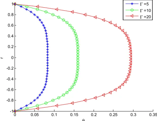
Γ =5 Γ =10 Γ =20

0 0.05 0.1 0.15 0.2 0.25 0.3 0.35

-1 -0.8 -0.6 -0.4 -0.2 0 0.2 0.4 0.6 0.8 1

w

r

(10)

Figure 11. Effect of varying parameter To on the velocity distribution of Reynolds viscosity model when for Λ = δ =γ= C =Γ =1

Figure 12. Effect of pressure gradient parameter C on the temperature distribution of Reynolds viscosity model under no slip condition when γ= Γ = Λ = δ = γ= 1.

Figure 13. Effect of varying parameter C for the temperature distribution of Reynolds viscosity model under slip condition when for Λ = δ = Γ =γ=1.

0 0.05 0.1 0.15 0.2 0.25 0.3 0.35

-1 -0.8 -0.6 -0.4 -0.2 0 0.2 0.4 0.6 0.8 1

w

r

To =0.5 To =0.8 To =1

0 0.002 0.004 0.006 0.008 0.01 0.012 0.014 0.016 0.018 -1

-0.8 -0.6 -0.4 -0.2 0 0.2 0.4 0.6 0.8 1

θ

r

C =-0.5 C =-0.75 C =-1

0.04 0.045 0.05 0.055 0.06 0.065 0.07 0.075 0.08 0.085 0.09 -1

-0.8 -0.6 -0.4 -0.2 0 0.2 0.4 0.6 0.8 1

θ

r

C =-0.5

(11)

Figure 14. Effect of varying parameter Γ on the temperature distribution of Reynolds viscosity model under no slip condition when γ= δ = Λ = -C = 1.

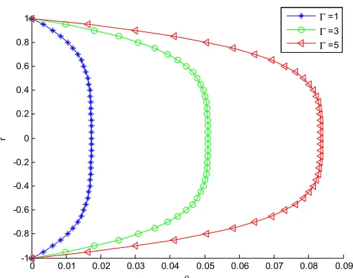
Figure 15. Effect of varying parameter Γ on the temperature distribution of Reynolds viscosity model under slip condition when for Λ = -C = δ =γ=1.

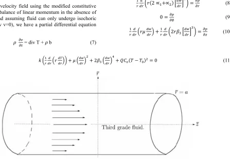
Figure 16. Effect of varying parameter Λon the temperature distribution of Reynolds viscosity model under no slip condition when γ= δ = Γ = -C = 1. 0 0.01 0.02 0.03 0.04 0.05 0.06 0.07 0.08 0.09

-1 -0.8 -0.6 -0.4 -0.2 0 0.2 0.4 0.6 0.8 1

θ

r

Γ =1 Γ =3 Γ =5

0.2 0.25 0.3 0.35 0.4 0.45 0.5

-1 -0.8 -0.6 -0.4 -0.2 0 0.2 0.4 0.6 0.8 1

θ

r

Γ =1.2

Γ =1.5

Γ =1.8

0 0.002 0.004 0.006 0.008 0.01 0.012 0.014 0.016 0.018 0.02 -1

-0.8 -0.6 -0.4 -0.2 0 0.2 0.4 0.6 0.8 1

θ

r

(12)

Figure 17. Effect of varying parameter Λ on the temperature distribution of Reynolds viscosity model under slip condition when for Γ = -C = δ =γ=1.

Figure 18. Effect of varying parameter γ on the temperature distribution of Reynolds viscosity model under no slip condition when δ = Λ = -C = 1.

Figure 19. Effect of varying parameter γ on the temperature distribution of Reynolds viscosity model under slip condition when for Λ = -C = δ =γ=1.

0.12 0.14 0.16 0.18 0.2 0.22 0.24

-1 -0.8 -0.6 -0.4 -0.2 0 0.2 0.4 0.6 0.8 1

θ

r

Λ =0 Λ =0.5 Λ =1

0 0.002 0.004 0.006 0.008 0.01 0.012 0.014 0.016 0.018 0.02 -1

-0.8 -0.6 -0.4 -0.2 0 0.2 0.4 0.6 0.8 1

θ

r

γ =-4 γ =0 γ =4

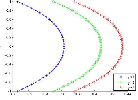
0.3 0.32 0.34 0.36 0.38 0.4 0.42 0.44

-1 -0.8 -0.6 -0.4 -0.2 0 0.2 0.4 0.6 0.8 1

θ

r

(13)

Figure 20. Effect of varying parameter A on the temperature distribution of Vogel’s viscosity model under no slip condition when B=Γ = Λ = δ =-C= To=1.

Figure 21. Effect of varying parameter A on the temperature distribution of Vogel’s viscosity model under slip condition when for B=Λ = δ = Γ =-C=To=1.

The shows the effect of pressure drop parameter, C for the Reynolds viscosity model on the velocity distribution in the pipe is shown in Figure 2. From the result, it shows that as the numerical value of C increases for no slip condition, the maximum velocity of the fluid which is at the center of the pipe but the fully developed velocity profile doesn’t begin at the origin which shows that there is a slip or no sticking of the fluid particle at the walls of the pipe. Increasing values of viscous dissipation (Γ) gives a corresponding increase in velocity distribution for the Reynolds viscosity model and viscous dissipation, Γ is maximum at the pipe center as depicted in Figure 3. The similar trends are recorded in the controlling parameters of the flow and heat transfer processes as shown in Figures 4-11.

Effects of slip on the temperature distribution are presented in Figures 12-32. Figures 12-19 show the effects of pressure drop parameter, C, viscous dissipation (Γ), viscosity variation parameter (γ), non-Newtonian material parameter of the fluid, Λfor the Reynolds’ viscosity model. It can be

seenthat as the fluid parameters increase, the temperature distribution increases and attains maximum value at the center of the pipe for bot no slip and slip conditions. However, the effects of slip shows that the curvesshift to the right and away from the origin i.e. the fully developed profile does not begin at the origin for the slip condition as shown in Figures 13, 15, 17 and 19. These same trends are displayed for the controlling for parameters of the fluid under Vogel’s viscosity model as shown in Figure 22-33. However, an opposed trend was recorded in parameter A. For increasing values of parameter A in the Vogel’s Viscosity model gives decreasing temperature distribution and the effect of the Vogel’s parameter A is maximum at the center of the pipe for both slip and no slip conditions shown in Figures 20 and 21

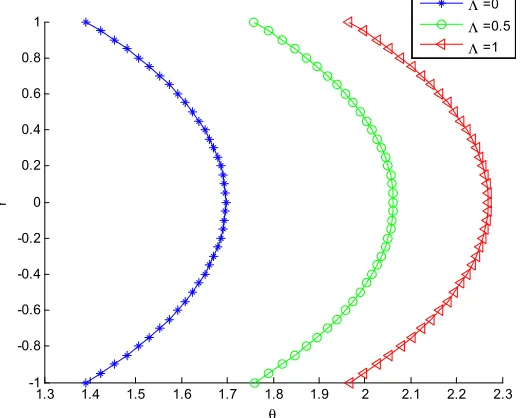
Also, the third grade fluid can be seen to exhibit Newtonian character for the Reynolds viscosity model when Λ= 0 and also the effect when the fluid behaves non Newtonian at increasing values of Λ. It can be seen from the Figures 26 and 27 that at increasing values of non-Newtonian parameter (Λ) for the

0 0.002 0.004 0.006 0.008 0.01 0.012 0.014 0.016 0.018 -1

-0.8 -0.6 -0.4 -0.2 0 0.2 0.4 0.6 0.8 1

θ

r

A =2 A =1.5

A =1

0.7 0.8 0.9 1 1.1 1.2 1.3 1.4

-1 -0.8 -0.6 -0.4 -0.2 0 0.2 0.4 0.6 0.8 1

θ

r

(14)

Vogel’s model gives increasing values of temperature distribution which maximum effect occurs at center of the pipe.

Figure 22. Effect of varying parameter C on the temperature distribution of Vogel’s viscosity model under no slip condition when B=Γ = Λ = δ =-C= To=1.

Figure 23. Effect of varying parameter δ on the temperature distribution of Vogel’s viscosity model under slip condition when for B=Λ = Γ =-C=To=1.

Figure 24. Effect of varying parameter Γ on the temperature distribution of Vogel’s viscosity model under no slip condition when B= Λ = δ =-C= To=1.

0 0.002 0.004 0.006 0.008 0.01 0.012 0.014 0.016 0.018 -1

-0.8 -0.6 -0.4 -0.2 0 0.2 0.4 0.6 0.8 1

θ

r

C =-0.5 C =-0.75 C =-1

1.4 1.5 1.6 1.7 1.8 1.9 2 2.1 2.2 2.3 2.4 -1

-0.8 -0.6 -0.4 -0.2 0 0.2 0.4 0.6 0.8 1

θ

r

C =-0.5 C =-0.7 C =-1

0 0.05 0.1 0.15 0.2 0.25 0.3 0.35

-1 -0.8 -0.6 -0.4 -0.2 0 0.2 0.4 0.6 0.8 1

θ

r

Γ =5

Γ =10

(15)

Figure 25. Effect of varying parameter Γ on the temperature distribution of Vogel’s viscosity model under slip condition when for B= δ = Γ =-C=To=1.

Figure 26. Effect of varying parameter Λ on the temperature distribution of Vogel’s viscosity model under no slip condition when B= Γ = δ =-C= To=1.

Figure 27. Effect of varying parameter Λ on the temperature distribution of Vogel’s viscosity model under slip condition when for B= δ = Γ =-C=To=1.

1.8 2 2.2 2.4 2.6 2.8 3 3.2 3.4 3.6 3.8 -1

-0.8 -0.6 -0.4 -0.2 0 0.2 0.4 0.6 0.8 1

θ

r

Γ =1 Γ =1.2 Γ =1.4

0 0.002 0.004 0.006 0.008 0.01 0.012 0.014 0.016 0.018 -1

-0.8 -0.6 -0.4 -0.2 0 0.2 0.4 0.6 0.8 1

θ

r

Λ =0

Λ =0.5

Λ =1

1.3 1.4 1.5 1.6 1.7 1.8 1.9 2 2.1 2.2 2.3

-1 -0.8 -0.6 -0.4 -0.2 0 0.2 0.4 0.6 0.8 1

θ

r

(16)

Figure 28. Effect of varying parameter B on the temperature distribution of Vogel’s viscosity model under no slip condition when A=Γ = Λ = δ =-C= To=1.

Figure 29. Effect of varying parameter B on the temperature distribution of Vogel’s viscosity model under slip condition when for A=Λ = δ = Γ =-C=To=1.

Figure 30. Effect of varying parameter To on the temperature distribution of Reynolds viscosity model under no slip condition when γ= δ = Λ = -C = 1.

0 0.002 0.004 0.006 0.008 0.01 0.012 0.014 0.016 0.018 -1

-0.8 -0.6 -0.4 -0.2 0 0.2 0.4 0.6 0.8 1

θ

r

B =0.5 B =0.8 B =1

1.8 2 2.2 2.4 2.6 2.8 3

-1 -0.8 -0.6 -0.4 -0.2 0 0.2 0.4 0.6 0.8 1

θ

r

B =1 B =1.5 B =2

0 0.002 0.004 0.006 0.008 0.01 0.012 0.014 0.016 0.018 -1

-0.8 -0.6 -0.4 -0.2 0 0.2 0.4 0.6 0.8 1

θ

r

(17)

Figure 31. Effect of varying parameter To on the temperature distribution of Vogel’s viscosity model under slip condition when for Λ = -C = δ =γ=1.

Figure 32. Effect of varying parameter δ on the temperature distribution of Vogel’s viscosity model under no slip condition when γ= To = Λ = -C = 1.

Figure 33. Effect of varying parameter δ on the temperature distribution of Vogel’s viscosity model under slip condition when γ= To = Λ = -C = 1.

1.1 1.15 1.2 1.25 1.3 1.35 1.4 1.45 1.5 1.55 1.6 -1

-0.8 -0.6 -0.4 -0.2 0 0.2 0.4 0.6 0.8 1

θ

r

To =0.5 To =0.6

To =0.7

0.004 0.006 0.008 0.01 0.012 0.014 0.016 0.018 0.02 -1

-0.8 -0.6 -0.4 -0.2 0 0.2 0.4 0.6 0.8 1

θ

r

δ =0 δ =0.5 δ =1

0.06 0.08 0.1 0.12 0.14 0.16 0.18 0.2 0.22 0.24 0.26 -1

-0.8 -0.6 -0.4 -0.2 0 0.2 0.4 0.6 0.8 1

θ

r

δ =0

δ =0.8

(18)

When heat generation term is excluded the effect is seen as δ=0. Figures 32 and 33 show the effects of temperature-dependent internal heat generation term for the Vogel’s viscosity model on the temperature distribution for linear temperature-dependent heat source. From the figures, it shows that as δ increases, the temperature distribution of the fluid increases. This behaviour is due to the fact that the heat generation mechanism creates a layer of hot fluid and at some level when the internal heat generation parameter is relative large, the resulting temperature of the fluid finally exceeds the least temperature distribution in the pipe [12].

Table 1. Comparison of Results for Reynold’s Model.

Γ θmax (FDM) θmax (Perturbation) Absolute Diffrence

5 0.0850 0.0846 0.0004

10 0.1780 0.1783 0.0003

15 0.2565 0.2570 0.0005

20 0.4310 0.4305 0.0005

Table 2. Comparison of Results for Reynold’s Model.

Λ θmax (FDM) θmax (Perturbation) Absolute Diffrence

0 0.0185 0.0188 0.0003

5 0.0138 0.0140 0.0002

10 0.0085 0.0087 0.0002

15 0.0120 0.0116 0.0004

Table 3. Comparison of Results for Vogel’s Model.

A θmax (FDM) θmax (Perturbation) Absolute Diffrence

1 0.0168 0.0170 0.0002

2 0.0068 0.0070 0.0002

3 0. 0029 0.0030 0.0001

4 0.0010 0.0010 0.0000

Tables 1-3 show the comparison of the results of finite difference method (FDM) and the perturbation method. The Tables show good agreement between the two results. The observed discrepancy might be due to the linearized boundary conditions.

5. Conclusion

In this work, nonlinear analysis of heat transfer in a pipe flow of a third grade fluid with temperature-dependent viscosities and heat generation under non-linear slip boundary conditions has been carried out using perturbation technique. The obtained approximate solutions of the linear and quadratic temperature-dependent heat generation have been used to investigate the effects of the model parameters on the flow and heat transfer in the third grade fluid. The results can be used to advance the analysis and study of the behaviour of third grade fluid flow and steady state heat transfer processes such as found in coal slurries, polymer solutions, textiles, ceramics, catalytic reactors, oil recovery applications etc.

Nomenclature

a and b Constant from dimensional Vogel’s viscosity model

M Constant from dimensional Reynold’s viscosity model

A= a/ (Dššš_™β) Dimensionless constant from Vogel’s viscosity model

B= (b +Dššš_™)/ (Dšššβ_™ ) Dimensionless constant from Vogel’s viscosity model

B™ Initial concentration of reacting species

C= (H //_CœG_C) (•pŸ_•ž Pressure gradient parameter

K Constant thermal conductivity

•p_Ÿ_• _{Pressure gradient along the normal to the pipe axis}

•p •ž

Ÿ Pressure gradient in the axial direction

•p •

Ÿ Pressure gradient in rotational direction

Q Heat generation constant

r Dimensional perpendicular distance in pipe axis

̅

= r/ R Dimensionless perpendicular distance in pipe axis

R Radius of the pipe

D™

šššš Initial temperature

W(r) Dimensional velocity component in the z axis

G¢ = G /G_C Dimensionless velocity component in the z axis

GC Dimensional reference velocity

z Axis of the cylinder

, , Constant material constant

β = RDššš_™/E Activation energy

γ = MβDššš_™ Reynolds viscosity variational parameter

/ Dynamic shear viscosity

μš= / //_Cœ Dimensionless viscosity

(19)

Γ = 4/_CœG_C/ (KDššš_™β) Viscous heating parameter θ= (T - D_™) E/ (RDššššš_™ ) Dimensionless temperature excess

Λ= β G_C/ (/_Cœ_C) Non-Newtonian material parameter of the fluid

δ = QE _™H B_™/ (RKDššššš_™ ) Heat generation parameter

References

[1] R. L. Fosdick and K. R. Rajagopal Thermodynamics and stability of fluids of third grade, Procter Society London, volume 339 (1980), 351-377.

[2] S. N. Majhi and V. R. Nair Flow of a third grade fluid over a sternosed tubes, Indian national science academy, volume 60 (3) (1994), 535.

[3] M. Massoudi and I. Christie Effects of variable viscosity and viscous dissipation on the flow of a third grade fluid in a pipe, International journal of nonlinear mechanics, volume 30 (1995) 687.

[4] M. Yurusoy M. and Pakdemirli. Approximate analytical solution for the flow of a third grade fluid in a pipe, International journal of nonlinear mechanics, volume 37 (2002). 187-195.

[5] K. Vajrevelu, J. r. Cannon, D. Rollins and J. Leto on solutions of some non-Linear differential equations arising in third grade fluid flows, International journal of engineering science, volume 40 (2002), 1791.

[6] T. Hayat, S. Nadeem, S. Asghar, and A. M. Siddiqui. Fluctuating flow of a third order fluid on a porous plate in a rotating medium, International journal of nonlinear mechanics, volume 36 (2002), 901-916.

[7] Y. Muhammet. Similarity solutions to boundary layer equations for third grade non-Newtonian fluid in special channel coordinate system, Journal of theoretical and applied mechanics, volume 41 (4) (2003) 775-787.

[8] M. Yurusoy. Flow of a third grade fluid between concentric cylinder, Journal of mathematical and computational applications, volume 9 (1) (2004), 11-12.

[9] M. Pakdemirli and B. S. Yilbas Entropy generation for a pipe flow of a third grade fluid with Vogel model viscosity, International journal of nonlinear mechanics, volume 43 (3) (2006). 432-437.

[10] M. Sajid, R. Mahmood and T. Hayat (2008) Finite element solution for flow of a third grade fluid past a horizontal porous plate with partial slip, International journal for computer and mathematics with applications, volume 56, 1236.

[11] R. Elahi, T. Hayat, F. M. Mahomed and S. Asghar. Effects of slip on the nonlinear flow of the third grade fluid, Journal of the nonlinear analysis, volume 11, (2010) 139-146.

[12] O. J. Jayeoba, and S. S. Okoya. Approximate analytical solutions for pipe flow of a third grade fluid with variable model of viscosities and heat generation/absorption, Journal of the Nigerian mathematical society, volume 31 (2012), 207-227.

[13] B. Y. Ogunmola, A. T. Akinshilo and M. G. Sobamowo. Perturbation Solutions for Hagen–Poiseuille Flow and Heat transfer of Third Grade Fluid with Temperature-Dependent

Viscosities and Internal Heat Generation. Article in Press, International Journal of Engineering Mathematics, Hindawi, 2016.

[14] S. S. Abbasbandy, T. Hayat, R. Ellahi and S. Asghar. Numerical results of a flow in third grade fluid between two porous walls, Verlagderzeitschrift fur Naturforschurg, volume 0932 (2008), 51.

[15] I. Nayak, A. K. Nayak and J. Padhy Numerical solutions for the flow and heat transfer of a third grade fluid past a porous vertical plate, Journal for advanced studies theoretical physics, volume 6, (2012), 615.

[16] Y. M. Aiyesimi, G. T. Okedayo and O. W. Lawal. Unsteady magneto hydrodynamic (MHD) thin film flow of a third grade fluid with heat transfer and no slip boundary condition down an inclined plane, International journal of physical sciences, volume 8 (19) (2013), 946.

[17] A. W. Ogunsola and B. A. Peter. Effect of variable viscosity on third grade fluid flow over a radiative surface with Arrhenius reaction, International journal of pure and applied sciences and technology, Volume 22 (1) (2014), 1-2.

[18] M. Yurusoy, M. Pakdemirli and B. S. Yilbas. Perturbation solution for third grade fluid flowing between parallel plates, Proceedings of the institute of Mechanical Engineering, volume 222 Part C, (2007). 653.

[19] M. G. Sobamowo, L. O. Jayesimi and M. A. Waheed. Magnetohydrodynamic squeezing flow analysis of nanofluid under the effect of slip boundary conditions using variation of parameter method. Karbala International Journal of Modern Science. volume 4 (2018), 107-118.

[20] M. G. Sobamowo, A. T. Akinshilo and A. A. Yinusa. Thermo-Magneto-Solutal Squeezing Flow of Nanofluid between Two Parallel Disks Embedded in a Porous Medium: Effects of Nanoparticle Geometry, Slip, and Temperature Jump Conditions. Modeling and Simulation in Engineering. volume 2018, Article ID 7364634, 18 pages.

[21] M. G. Sobamowo, L. O. Jayesimi and M. A. Waheed. Axisymmetric Magnetohydrodynamic Squeezing flow of nanofluid in a porous medium under the influence of slip boundary conditions. Transport Phenomena in nano and micro Scales. volume 6 (2) (2018), 122-132.

[22] M. G. Sobamowo and A. T. Akinshilo. Analysis of flow, heat transfer and entropy generation in a pipe conveying fourth grade fluid with temperature-dependent viscosities and internal heat generation. Journal of Molecular Liquids, volume 241 (2018), 188-198.

[23] M. G. Sobamowo. Singular perturbation and differential transform methods to two-dimensional flow of nanofluid in a porous channel with expanding/contracting walls subjected to a uniform transverse magnetic field. Thermal Science and Engineering Progress. volume 4 (2017), 71-84.

(20)

[25] M. G. Sobamowo and L. O. Jayesimi. Squeezing flow analysis of nanofluid under the effects of magnetic field and slip boundary using Chebychev spectral collocation method. Fluid Mechanics. volume 3 (6) (2017).

[26] M. G. Sobamowo, L. O. Jayesimi and M. A. Waheed (2017). On the Squeezing flow of nanofluid through a porous medium with slip boundary and magnetic field: A comparative study of

three approximate analytical methods. Global Journal of Engineering, volume 17 (6), 61-76.