Published online September 30, 2014 (http://www.sciencepublishinggroup.com/j/ajam) doi: 10.11648/j.ajam.20140205.12
ISSN: 2330-0043 (Print); ISSN: 2330-006X (Online)
Modified midpoint method for solving system of linear
Fredholm integral equations of the second kind
Salam Jasim Majeed
Department of Physics, College of Science, University of Thi-Qar, Thi-Qar, Iraq
Email address:
To cite this article:
Salam Jasim Majeed. Modified Midpoint Method for Solving System of Linear Fredholm Integral Equations of the Second Kind. American Journal of Applied Mathematics. Vol. 2, No. 5, 2014, pp. 155-161. doi: 10.11648/j.ajam.20140205.12
Abstract:
In this paper numerical solution to system of linear Fredholm integral equations by modified midpoint method is considered. This method transforms the system of linear Fredholm integral equations into a system of linear algebraic equations that can be solved easily with any of the usual methods. Finally, some illustrative examples are presented to test this method and the results reveal that this method is very effective and convenient by comparison with exact solution and with other numerical methods such as midpoint method, trapezoidal method, Simpson's method and modified trapezoidal method.All results are computed by using a programs written in Matlab R2012b
.
Keywords:
System of Fredholm Integral Equations, Modified Midpoint Method1. Introduction
Mathematical modeling for many problems in different disciplines, such as engineering, chemistry, physics and biology leads to integral equation, or system of integral equations. Most differential equations can be expressed as integral equations. Also, a system of differential equations can be written as a system of integral equations, [1, 2]. For these reasons the great interest for solving these equations. Since these equations usually cannot be solved explicitly, so the numerical solutions have been highly studied by many authors, [1-4].
Now we consider the following systems of linear Fredholm integral equation of the second kind:
b a
U(x)=F(x)+
∫
K(x, y)U(y)dy, x∈[a, b]. (1.1)where
[
]
[
]
T
1 2 m
T
1 2 m
ij
U(x) u (x), u (x), , u(x) ,
F(x) f (x), f (x), , f (x) ,
K(x, y) k (x, y) , i, j 1(1)(m).
= =
= =
…
…
In system (1.1) the known kernel K(x, y) is continuous, the function F(x) is given, and U(x) is the solution to be determined. There are several numerical methods for solving this system. For example, Rationalized Haar functions
method [5], Block–Pulse functions method[6], Expansion methods [7, 8], Decompostion method [9] and Orthogonal Triangular functions method [10].
In recent years, a new class of quadrature formulas are introduced called as modified (corrected) Newton-Cotes formula which based on derivatives of the function. The uses of modified quadrature formula for solving integral equations and their systems have been considered by many authors: modified trapezoidal [11-13 ], modified Simpson’s [13-16 ] and modified midpoint method [17].
In this paper, we want to find the numerical solution for the system given by eq (1.1) by using the repeated modified midpoint formula for definite integral:
[
]
2
b n
j j 1 a
4 7h (b a) (4)
f ( ). 5760
h
f (x)dx h f (x ) f (a) f (b) 24
=
− +
′ ′
=
∑
+ −∫
η (1.2)where n is the number of subinterval of [a, b],
b a
h n , x a ( j 1 / 2)h, j 1(1)n j
−
= = + − = and η∈(a, b).
To do this, we assume the functions k (x,y)ij
x ∂
∂ ,
k (x,y)ij y
∂ ∂
and f (x)i′ exist for all i, j=1(1)m.
2. Modified Midpoint Method
Consider the ith equation of system (1.1)
m b
i i ij j
a j 1
u (x) f (x) k (x, y)u (y)dy ,
=
= +
∑∫
i=1(1)m (2.1)To solve eq. (2.1), we approximate the integral part that appeared in the right hand side by the repeated modified midpoint formula to get,
)
ij 0 j 0 ij n 1 j n 1 ij n 1 j n 1
k (x, x )u (x ) J (x, x′ + )u (x + ) k (x, x + )u (x′ + ),
+ − −
(2.2)
where, x0 =a, xn 1+ =b and ij
ij
k (x, y)
J (x, y) ,
y ∂
= ∂ i, j 1(1)m= .
Hence for
x
=
x ,
r r=0(1)(n+1), we get the following system of equations:(
2m n h
ir ir j 1 s 1 ijrs js 24 ijr0 j0
u f h k u J u
= =
= +
∑
∑
+)
ijr0 j0 ijr n 1 jn 1 ijr n 1 jn 1
k u′ J + u + k + u′ +
+ − − (2.3)
where
ir i r
u
=
u (x ),
f
ir=
f (x ),
i ri0 i 0 in 1 i n 1
u
′
=
u (x ), u
′
′
+=
u (x
′
+),
ijrs ij r s
J
=
J (x , x ),
kijrs =k (x , x )ij r s .If we differential both sides of equation (2.1) with respect
to x and setting H (x, y)ij = k (x,y)ij x
∂
∂ one can obtain:
b m
i i j 1 a ij j
u (x) f (x) H (x, y)u (y)dy, i 1(1)m
=
′ = ′ +
∑ ∫
= . (2.4)We note that if u a solution of eq.(2.1) then it is a solution of eq.(2.4) too. Now, for solving eq.(2.4), we must
consider two cases, and for simplify let L (x, y)
ij =
2
y
k (x,y)ij x∂
∂
∂ .
Case 1: The partial derivatives Lij( , )x y exists for each
{
}
, ∈ 1, 2,...,
i j m .
In this case, we approximate the integral part that appeared in the right hand side of eq.(2.4) by the repeated modified midpoint formula to get,
(
)
2m n h
i i j 1 s 1 ij s j s 24 ij 0 j 0 ij 0 j 0 ij n 1 j n 1 ij n 1 j n 1
u (x) f (x) h H (x, x )u (x ) L (x, x )u (x )
H (x, x )u (x ) L (x, x )u (x ) H (x, x )u (x )
= = + + + + ′ = ′ + + ′ ′ + − −
∑
∑
(2.5)By setting
x
=
x ,
r r=0(1)(n+1) in eq.(2.5), one canget
2
m h n
ir ir j 1 24 ijr0 j0 s 1 ijrs js
u f L u h H u
= = ′ = ′ +
∑
+∑
(
)
2 2 h hijr n 1 jn 1 ijr0 j0 ijr n 1 jn 1
24L + u + 24 H u H + u +
′ ′
− + −
(2.6)
where
ir i r
f′ =f (x )′ , Hijrs=H (x , x )ij r s and Lijrs=L (x , x )ij r s .
From eq.(2.6) and eq.(2.3) one can get the following system which consist of m(n+4) equations and m(n+4) unknowns:
{
u , u ,..., ui0 i1 in 1+ , u , u′i0 in 1′ +}
, i=1(1)m.(
)
(
)
2 2 2
2 2 2
2
m h n h h
ir ir j 1 24 ijr 0 j0 s 1 ijrs js 24 ijr n 1 jn 1 24 ijr 0 j0 ijr n 1 jn 1
m h n h h
i0 i0 j 1 24 ij00 j0 s 1 ij0s js 24 ij0n 1 jn 1 24 ij00 j0 ij0 n 1 jn 1
h
in 1 in 1 24
u
f
J
u
h
k u
J
u
k
u
k
u
,
u
f
L
u
h
H
u
L
u
H
u
H
u
,
u
f
+ + + + = = + + + + = = + +
′
′
=
+
+
−
+
−
′
=
′
+
+
−
+
′
−
′
′
=
′
+
∑
∑
∑
∑
(
)
2 2m n h h
ijn 10 j0 ijn 1s js 24 ijn 1n 1 jn 1 24 ijn 10 j0 ijn 1n 1 jn 1
j 1=
L
+u
h
s 1=H
+u
L
+ +u
+H
+u
H
+ +u
+
+
−
+
′
−
′
∑
∑
(2.7)By solving the above system the numerical solutions of eq.(2.1) are obtained.
Case 2:The partial derivatives Lij( , )x y does not exist. In this case, we approximate the integral part that appeared in the right hand side of eq. (2.4) by the repeated midpoint formula to get,
( )
m n
i i ij s j s
j 1 s 1
u (x) f (x) h H (x, x )u (x ) , i 1 1 m.
= =
′ = ′ +
∑ ∑
= (2.8)By setting
0 1 n 1
x
=
x , x ,
…
, x
+,
in eq.(2.8), one can get:m n
ir ir j 1 s 1 ijrs js
u
′
= +
f
′
h
∑ ∑
= =H u
, r=0(1)(n+1). (2.9)From eq.(2.9) and eq.(2.3) one can get the following system which consists of m(n+4) equations and m(n+4) unknowns:
(
2m n h
i i j 1 s 1 ij s j s 24 ij 0 j 0
u (x) f (x) h k (x, x )u (x ) J (x, x )u (x )
= =
(
)
( )
( )
2 2 2
m h n h h
ir i r j 1 24 ijr 0 j0 s 1 ijrs js 24 ijr n 1 jn 1 24 ijr 0 j0 ijr n 1 jn 1
m n
i0 i0 j 1 s 1 ijr0 j0
m n
in 1 in 1 j 1 s 1 ijr n 1 jn 1
u
f
J
u
h
k u
J
u
k
u
k
u
,
u
f
h
H
u ,
u
f
h
H
u
,
i
1 1 m, r
0 1 (n 1).
+ + + +
= =
= =
+ + = = + +
=
+
+
−
+
′
−
′
′
′
=
+
′
=
′
+
=
=
+
∑
∑
∑ ∑
∑ ∑
(2.10)By solving the system given by eq. (2.10), the numerical solutions of eq.(2.1) are obtained.
3. Numerical Examples
In this section we give three numerical examples to test the Modified Midpoint method for solving system of linear Fredholm integral equations of the second kind. All results are computed by using a programs written in Matlab R2012b. In order to show the efficiency and high accuracy of the present method we compared the results with the exact solutions numerically in the tables (1-4). Also, we compared the error functions which obtained by our method and other numerical methods such as Midpoint, Trapezoidal, Simpson’s and Modified Trapezoidal graphically in the figures (1-4). Finally, the following notations are used in the tables and figures.
( ) Exact Solution
( ) Approximation solution
MMP(I) Modified Midpoint method case 1, eq.(2.7)
MMP(II) Modified Midpoint method case 2, eq.(2.10)
MT Modified Trapezoidal method
MP Midpoint method
T Trapezoidal method
S Simpson’s method
n Number of subinterval
and the error function is given by :
( ) = | ( ) − ( )|.
Example 1:
Consider the following system of linear Fredholm integral equations of the second kind, [12]
( )
(
)
2 2
1 1 2
2 4 2
2 1 2
1 1
25 5
12 6 0 0
1 1
7 1
12 5 0 0
u (x) 1 x x x 1 y u (y)dy x y u (y)dy u (x) x x x xy u (y)dy x xy u (y)dy
= − + + + +
= − − + + + −
∫
∫
∫
∫
(3.1)where the exact solution
(
) (
2 4)
1 2
u (x), u (x) = x +1, x and the
partial derivative L (x, y) exists. Therefore, this system can ij
be solved by using MMP(I) and the results presented in table 1 and fig. 1.
Table 1. The numerical results for example 1 with n=10 and n=30.
x ( ) ( ) ( ) ( )
n=10 n=30 n=10 n=30
0 1 1 1 0 0 0
0.05 1.00250000 1.00250190 1.00250002 0.00000625 0.00000649 0.00000625 0.15 1.02250000 1.02250586 1.02250007 0.00050625 0.00050709 0.00050626 0.25 1.06250000 1.06251004 1.06250012 0.00390625 0.00390785 0.00390627 0.35 1.12250000 1.12251443 1.12250018 0.01500625 0.01500876 0.01500628 0.45 1.20250000 1.20251904 1.20250024 0.04100625 0.04100982 0.04100629 0.55 1.30250000 1.30252386 1.30250029 0.09150625 0.09151104 0.09150631 0.65 1.42250000 1.42252889 1.42250036 0.17850625 0.17851241 0.17850633 0.75 1.56250000 1.56253414 1.56250042 0.31640625 0.31641394 0.31640634 0.85 1.72250000 1.72253960 1.72250049 0.52200625 0.52201562 0.52200637 0.95 1.90250000 1.90254527 1.90250056 0.81450625 0.81451746 0.81450639
Fig. 1. The error function via MMP(I), MP, T, S and MT for example 1 with n=10.
Example 2:
Consider the following system of linear Fredholm integral equations of the second kind:
1 1
x x y (x 2) y
1 0 1 0 2
1 1
x x xy (x y)
2 0 1 0 2
x 1 e 1
x 1 x 1 e 1
x 1
u (x) 2e e u (y)dy e u (y)dy
u (x) e e e u (y)dy e u (y)dy
− +
− +
+ − +
+ − +
= + − −
= + + − −
∫
∫
∫
∫
(3.2)
This system of integral equations has been solved by Block-Plus Function (BPF) in [6] and the exact solution is
(
)
(
x x)
1 2
u (x), u (x) = e , e− . Also the partial derivative L (x, y) ij
exists. Therefore, similar to example 1 this system can be solved by using MMP(I) and the results presented in fig. 2 and tables 2 and 3.
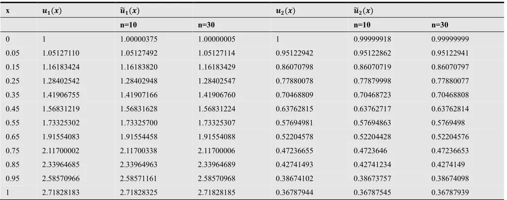
Table 2. The numerical results for example 2 with n=10 and n=30.
x ( ) ( ) ( ) ( )
n=10 n=30 n=10 n=30
0 1 1.00000375 1.00000005 1 0.99999918 0.99999999
0.05 1.05127110 1.05127492 1.05127114 0.95122942 0.95122862 0.95122941 0.15 1.16183424 1.16183820 1.16183429 0.86070798 0.86070719 0.86070797 0.25 1.28402542 1.28402948 1.28402547 0.77880078 0.77879998 0.77880077 0.35 1.41906755 1.41907166 1.41906760 0.70468809 0.70468723 0.70468808 0.45 1.56831219 1.56831628 1.56831224 0.63762815 0.63762717 0.63762814 0.55 1.73325302 1.73325700 1.73325307 0.57694981 0.57694863 0.5769498 0.65 1.91554083 1.91554458 1.91554088 0.52204578 0.52204428 0.52204576 0.75 2.11700002 2.11700338 2.11700006 0.47236655 0.4723646 0.47236653 0.85 2.33964685 2.33964963 2.33964689 0.42741493 0.42741234 0.4274149 0.95 2.58570966 2.58571161 2.58570968 0.38674102 0.38673757 0.38674098 1 2.71828183 2.71828325 2.71828185 0.36787944 0.36787545 0.36787939
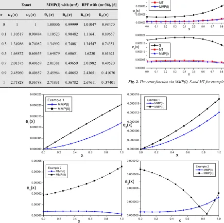
In table 3 we list the results obtained by MMP(I) with n=5 and compared with BPF results given in [6] at m=36. As we see from this table, it is clear that the result obtained by the present method is better than the results obtained by BPF method.
Moreover the Results of example 1 and 2 by MMP(I) and MMP(II) together are plotted in fig. 3 and show that MMP(I) solves system (1.1) more accurately than MMP(II), because in MMP(I) we use modified midpoint method for solving eq.(2.4) instead midpoint method.
0.0 0.1 0.2 0.3 0.4 0.5 0.6 0.7 0.8 0.9 1.0 0.00000
0.00006 0.00012 0.00018 0.00024
e1(x)
x
S MT MMP(I)
0.0 0.1 0.2 0.3 0.4 0.5 0.6 0.7 0.8 0.9 1.0 0.000
0.025 0.050 0.075 0.100
e1(x)
x
T MP MMP(I)
0.0 0.1 0.2 0.3 0.4 0.5 0.6 0.7 0.8 0.9 1.0 0.00000
0.00002 0.00004 0.00006
e2(x)
x
S MT MMP(I)
0.0 0.1 0.2 0.3 0.4 0.5 0.6 0.7 0.8 0.9 1.0 0.000
0.012 0.024 0.036
T MP MMP(I)
e2(x)
Table 3. The numerical solutions for example 2 obtained by MMP(I) and BPF , [6] with exact solutions.
Exact MMP(I) with (n=5) BPF with (m=36), [6]
( ) ( ) ( ) ( ) ( ) ( )
0 1 1 1.00006 0.99999 1.01047 0.98470
0.1 1.10517 0.90484 1.10523 0.90482 1.11641 0.89657
0.3 1.34986 0.74082 1.34992 0.74081 1.34547 0.74351
0.5 1.64872 0.60653 1.64879 0.60651 1.6230 0.61621
0.7 2.01375 0.49659 2.01381 0.49659 2.01982 0.49520 0.9 2.45960 0.40657 2.45964 0.40652 2.43651 0 .41070
1 2.71828 0.36788 2.71831 0.36782 2.67611 0 .37401 Fig. 2. The error function via MMP(I), S and MT for example 2 with n=10.
Fig. 3. Comparsin error functions via MMP(I), S and MT for example 1 and 2 with n=10.
Example 3:
Consider the following system of linear Fredholm integral equations of the second kind:
3/ 2 2
1 1 2
4 3
2 2 2
1 1
1
0 0
1 1
1
0 0
u (x) f (x) (x y) u (y)dy (x y) u (y)dy
u (x) f (x) (x y) u (y)dy (x y) u (y)dy
= − + − −
= − − − −
∫
∫
∫
∫
(3.3)where
2 9/ 2 1
7 7 11 16
60 30 12 315
f (x)= − + x+ x + x
9/ 2 7/ 2 2 5/ 2
(x 1) x(x 1) x (x 1) ,
2 4 2
9 7 5
− + + + − +
2 3 4
2
1 41 3 32 1
30 60 20 12 3
f (x)= − − x+ x + x − x .
and the exact solution
(
)
(
2 2 3)
1 2
u (x), u (x) = x ,− +x x +x .
In this system, we note that L (x, y)11 =−43(x+y)−1/2 not exists at (x, y)=(0, 0). Therefore, we used MMP(II) to solve this system and the results presented in table 4 and fig. 4.
0.0 0.1 0.2 0.3 0.4 0.5 0.6 0.7 0.8 0.9 1.0 0.000000
0.000005 0.000010 0.000015 0.000020
e1(x)
x S
MT MMP(I)
0.0 0.1 0.2 0.3 0.4 0.5 0.6 0.7 0.8 0.9 1.0 0.000000
0.000005 0.000010 0.000015 0.000020
e
2(x)
x S
MT MMP(I)
0.0 0.2 0.4 0.6 0.8 1.0 0.000000
0.000005 0.000010 0.000015 0.000020 0.000025
e
1(x)
x
Example 1 MMP(I) MMP(II)
0.0 0.2 0.4 0.6 0.8 1.0 0.000000
0.000003 0.000006 0.000009 0.000012 0.000015 0.000018
e
2(x)
x
Example 1 MMP(I) MMP(II)
0.0 0.2 0.4 0.6 0.8 1.0 0.00000
0.00001 0.00002 0.00003 0.00004 0.00005
e
1(x)
x
Example 2 MMP(I) MMP(II)
0.0 0.2 0.4 0.6 0.8 1.0 0.000000
0.000003 0.000006 0.000009 0.000012
e
2(x)
x
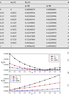
Table 4. The numerical results for example 3 with n=10 and n=30.
x ( ) ( ) ( ) ( )
n=10 n=30 n=10 n=30 0 0 0.00000078 0.00000001 0 -0.00001061 -0.00000013 0.05 0.0025 0.00249936 0.00249999 -0.047375 -0.04738417 -0.04737511 0.15 0.0225 0.02249644 0.02249996 -0.124125 -0.12413184 -0.12412508 0.25 0.0625 0.06249333 0.06249992 -0.171875 -0.17188006 -0.17187506 0.35 0.1225 0.12249003 0.12249988 -0.184625 -0.18462864 -0.18462505 0.45 0.2025 0.20248653 0.20249983 -0.156375 -0.15637746 -0.15637503 0.55 0.3025 0.30248283 0.30249979 -0.081125 -0.08112641 -0.08112502 0.65 0.4225 0.42247895 0.42249974 0.047125 0.04712456 0.04712499 0.75 0.5625 0.56247488 0.56249969 0.234375 0.23437545 0.23437501 0.85 0.7225 0.72247064 0.72249965 0.486625 0.48662621 0.48662501 0.95 0.9025 0.90246621 0.90249958 0.809875 0.80987678 0.80987502
1 1 0.99996393 0.99999955 1 1.00000196 1.00000002
Fig. 4. The error function via MMP(I), S and MT for example 3 with n=10.
4. Conclusions
Modified Midpoint method is applied to the numerical solution for solving system of linear Fredholm integral equations. Numerical results, compared with other methods such as the midpoint, Trapezoidal, Simpson, Modified Trapezoidal and Block Plus Function method, show that the presented method is of higher precision and from the illustrative tables, we conclude that when the number of subintervals n is increased we can obtain a very good accuracy. Also as can be seen from Table 3, MMP(I) is better than MMP(II) for solving system (1.1) .
References
[1] Rmp.P. Kanwal, ‘‘Linear Integral Equations, Theory and Technique’’, Academic press, INC, 1971.
[2] T. A. Burton, "Volterra Integral and Differential Equations", second ed., Elsevier, Netherlands, 2005.
[3] K. E. Atkinson, ‘‘The Numerical Solution of Integral Equations of the Second Kind’’, Cambridge University Press, 1997.
[4] A. M. Wazwaz, ‘‘Linear and nonlinear integral equations: methods and applications’’, Higher education, Springer, 2011.. [5] K. Maleknejad, F. Mirzaee, Numerical solution of linear Fredholm integral equations system by rationalized Haar functions method, Int. J. Comput. Math. 80 (11) (2003) 1397– 1405.
[6] K. Maleknejad, M. Shahrezaee, H. Khatami, ‘‘Numerical solution of integral equations system of the second kind by Block–Pulse functions’’, J. Applied Mathematics and Computation, 166 (2005) 15–24.
[7] K. Maleknejad, N. Aghazadeh, M. Rabbani, ‘‘Numerical solution of second kind Fredholm integral equations system by using a Taylor-series expansion method’’, J. Appl. Math. and Comupt., Vol. 175, No. 2, 2006, pp 1229-1234.
[8] M. Rabbani, K. Maleknejad, N. Aghazadeh, ‘‘Numerical computational solution of the Volterra integral equations system of the second kind by using an expansion method’’, J. Appl. Math. and Comupt., Vol. 187, No. 2, 2007, pp 1143-1146.
[9] A. R. Vahidi, M. Mokhtari, A. R. Vahidi, ‘‘On the decomposition method for system of linear Fredholm integral equations of the Second Kind’’, J. Appl. Math. Scie., Vol. 2, No. 2, 2008, pp 57-62.
[10] E. Babolian, Z. Masouri, S. Hatamzadeh-Varmazyar, ‘‘A direct method for numerically solving integral equations system using orthogonal triangular functions’’, Int. J. Ind. Math. 01, No. 2, 2009, pp 135-145.
[11] J. S. Nadjafi, M. Heidari, ‘‘Solving Linear Integral Equations of the Second kind with Composed Modified Trapzoid Quadrature Method", J. Appl. Math. and Comupt., 189(4)(2007), 980-985.
[12] S. J. Majeed, ‘‘Modified Trapezoidal Method for Solving System of Linear Integral Equations of the Second Kind", J. Al-Nahrain University, 11(4)(2009), pp.131-134.
[13] S. J. Majeed, ‘‘Numerical Methods for Solving Linear Fredholm-Volterra Integro differential Equations of the Second Kind ", J. Al-Nahrain University, 13(2)(2010), pp. 194-204.
0.0 0.1 0.2 0.3 0.4 0.5 0.6 0.7 0.8 0.9 1.0
0.00000 0.00006 0.00012 0.00018 0.00024
e1(x)
x S
MT MMP
0.0 0.1 0.2 0.3 0.4 0.5 0.6 0.7 0.8 0.9 1.0
0.00000 0.00002 0.00004 0.00006
e2(x)
x
[14] S. J. Majeed, ‘‘Adapted Method for Solving Linear Volterra Integral Equations of the Second kind Using Corrected Simpson's Rule ", J. College of Education, Babylon University, Vol.5 (1), January, 2010, pp. 507-511.
[15] Farshid Mirzaee, Sima Piroozfar, "Numerical solution of linear Fredholm integral equations via modified Simpson’s quadrature rule", J. King Saud University (Science) (2011)23,7–10.
[16] Farshid Mirzaee, ‘‘A Computational Method for Solving Linear Volterra Integral Equations", J. Applied Mathematical Sciences, Vol. 6, no. 17, 2012, 807 - 814.
[17] S. J. Majeed, ‘‘Modified Midpoint Method For Solving Linear Fredholm Integral Equations Of The Second Kind ", J. Al Qadisiya for computers Science and mathematics, Vol.3 (1), 2011, pp.28-46.
[18] S. D. Conte, Carl de Boor, ‘‘Elementary Numerical Analysis An Algorithmic Approach’’, International series in pure and applied mathematics, McGraw-Hill Book Company, USA, 1980.
[19] J. Z. Christopher, ‘‘Numerical Analysis for Electrical and Computer Engineers’’, John Wiley & Sons, Inc., New Jersey, 2004.
[20] N. S. Barnett and S. S. Dragomir, ‘‘On the Perturbed Trapezoid Formula’’, RGMIA Research Report Collection, 4(2)(2001), Article 4.
[21] X. L. Cheng and J. Sun, "Note on the Perturbed Trapezoid Inequality’’, J. Inequality Pure Appl. Math., 3(2002), article 29, 1–7.
[22] N. Ujevi´c, "On Perturbed Mid-point and Trapezoid Inequalities and Applications’’, Kyungpook Math. J., 43(2003), 327-334.
[23] N. Ujevi´c and A. J. Roberts, ‘‘A Corrected Quadrature Formula and Applications’’, ANZIAM J., 45(E)(2004), 41-56.. [24] N. Ujevic´, ‘‘Generalization of the Corrected Mod-Point Rule and Error Bound’’, J. Computational Methods in Applied Mathematics, 5(1)(2005), pp 97–104.