New Solution of Factor Analysis Difference in Factor Product Combination

http://www.sciencepublishinggroup.com/j/jfa doi: 10.11648/j.jfa.20190706.11

ISSN: 2330-7331 (Print); ISSN: 2330-7323 (Online)

New Solution of Factor Analysis Difference in Factor

Product Combination

Liu Yun, Yonghong Yao, Qiaowen Yang

*

Hua Shang Accounting College, Guang Dong University of Finance and Economics, Guangzhou, China

Email address:

*_{Corresponding author}

To cite this article:

Liu Yun, Yonghong Yao, Qiaowen Yang. New Solution of Factor Analysis Difference in Factor Product Combination. Journal of Finance and Accounting. Vol. 7, No. 6, 2019, pp. 184-191. doi: 10.11648/j.jfa.20190706.11

Received: October 12, 2019; Accepted: November 7, 2019; Published: November 18, 2019

Abstract:

On the basis of the present situation and problems of factor analysis, this paper USES the methods of mathematical geometry and calculus to prove the interaction among factors when the factors in the two-factor and three-factor analysis equations are product function formulas. The exponential logarithmic scaling method is deduced and checked by calculation. The new factor analysis method can decompose the interaction between factors accurately and fairly. This approach is not limited to the analysis of differences between factors for the reporting period and the base period (actual and budgetary figures); In addition, it is a good way to decompose the interaction among factors by analyzing whether the differences among factors are increasing or decreasing. This provides an accurate basis for the success of retesting and adjusting the difference, and also provides a reliable basis for the attribution of the difference responsibility in the social and economic management activities. The correct factor analysis difference analysis, not only solved the long - time unresolved problems in economic management; It also solves the problem of comparative analysis of the difference between the success and failure of the experiment. The difference of factors determines the adjustment of the experiment. The correct difference analysis of factors plays a decisive role in the success of the reexperiment and has economic significance to improve the experimental results.

Keywords:

Factor Analysis, Decomposition of Interaction Difference, Exponential Logarithmic Proportionality

1. Introduction

We live in an era of rapid development of information technology and wide application of computers. In the era of cloud computing and big data, how our disciplines are connected with the application of modern tools, and how research methods are applied and Shared by each other. It is particularly important for modern intelligence to be widely integrated, constantly improved, integrated and innovated to adapt to the rapid changes and development. This paper studies propositions which are mainly different from existing methods. What is factor analysis? Factor analysis in the statistical analyzing the phenomenon refers to the use of statistical index system always changes in various factors affect the degree of a statistical analysis method, factor

analysis method to the financial management,

"management accounting", "financial cost management",

"financial analysis", "cost and management accounting", journal of applied statistics, the enterprise financial audit, occupies an important proportion in the textbook; Differential analysis of mathematical, chemical, physical and medical experiments is also commonly used.

management, accounting subject thesis is: the main factors (interpreted factors) and other factors (explain factors, also called factor) there is a proper relationship between correlation between factors, the main factors and factor between different experimental results of the overall difference, can be broken down into various factors affect the difference. The factor analysis method studied in this paper mainly refers to the product structure in the equation structure between factors, that is, the interaction between factors.

This paper is the second part after my book "analysis status of factor difference analysis in product structure of factor analysis", which is also the core content of solving the problems of factor analysis.

2. Problem Presentation

Taking the sales income (ω) = sales price (p)× sales quantity

(x) as an example, when analyzing the sales income factors in the reporting period and the base period:

The total difference is△ω=p1x1 -p0x0

Question:

1) in the serial substitution method of factor analysis, why are the substitution orders of factors different and the differences of factors' influences on the whole different? After this article solves the factor analysis solution, it will tell you that there is no "order hypothesis" in factor analysis where the substitution order changes and the calculation result changes.

In factor analysis, there is a combination of multiple factors. Taking two factors as an example, there is a combination of multiple factors whose difference is caused by interaction. In the balance calculation of factor analysis, why there are only three combinations in the combination of two factors, namely,

p1x1, p1x0, p0x0, or p1x1, p0x1, p0x0; Instead of four groups,

namely p1x1, p1x0, p0x1, p0x0?

2) the model of factor analysis is the continuous product structure, and there is an interaction between the factors. The difference analysis of explaining factors to the explained factors is made by using the elasticity coefficient in econometrics. Statistics USES the calculus principle to solve the incremental analysis of factors; Why "financial management", "financial analysis", "management accounting", "auditing", "cost management accounting", "financial cost management", etc.

3) can the difference of the influence of the interaction between factors in the factor analysis on the total difference be calculated? Increment is ok (xu guoxiang, statistics), what about factor analysis decrement? How to calculate multiple factors (professor xu guoxiang "statistics" has not solved)? Are there interactions? If there is, how to identify the extra difference?

4) can the current serial substitution and balance methods still be used? When the current analysis mode is product structure, the difference of factor influence between serial substitution and differential substitution in factor analysis is wrong, of course, the method is not available.

5) The correctness of the new factor analysis method and its nomenclature and application. This paper explores that the interaction between factors can also be apportioned. If there are several factors in the main factor, the influence will be several. There is no fictitious compound factor influence such as "structure", "rank" and "efficiency".

3. Interaction Verification

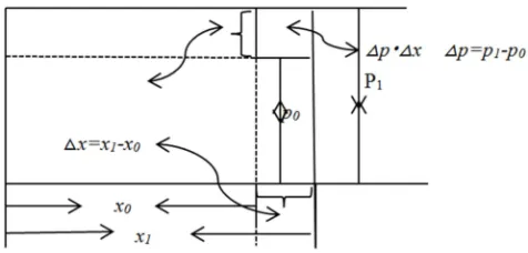
The product structure, the interaction between the factors (1) two-factor mathematical geometric area proof:

Figure 1. Differential graph of interaction of binary factors. 3.1. In The x

ω1=x1p1, ω0=x0p0, its area difference is changed to:

△ω=ω1-ω0=x1p1-x0p0

△ω=(△p + p0) (△x+x0)-p0x0

△ω=△px0+△xp0+△p△x (1) In the binary factor, its structure model is in the form of continuous product. When the influence of factor change on the population is the sum of the product of the base period number and variation difference of factor change and another factor times another variation difference. The product of the differences between two factors is called the interaction between the factors. Based on this, we can draw a conclusion: when the product structure of two factors, the change of one factor and the change of the other factor is called the factor interaction in factor analysis. Obvious:

In the continuous product structure model of factor analysis, the influence of factors on the whole is interactive.

Traditional factor analysis methods, serial substitution method and balance method (a simple method of serial substitution method), artificially add the influence difference of interaction delta p delta x to the difference of a factor, which leads to the calculation result, that is, the influence of each factor is not correct;

The attribution of the difference of the interaction according to the order of factor substitution.

3.2. Mathematical Calculus Proves That

(

)

(

)

(

2 2

)

(

) (

)

0, 0 0, 0 0 0 , 0 0, 0

p x

f p x p f p x x p x f p p x x f p x p x

p x

ω

ω

ω

′ ′ ∂ ∂

ωρ

∆ = ∆ + ∆ + ∆ + ∆ = + ∆ + ∆ − = ∆ + ∆ +

∂ ∂

If the function is

ω

= ⋅

p x

, the analysis of its increment is as follows:

(

) (

)

(

) (

)

0

0

0 0 0

0 0 0

,

|

,

|

p x

x p

f

p x

p x

x

x

p

f

p x

p x

p

p

x

ω

ω

∂

=

′

=

⋅

′

=

=

∂

∂

=

′

=

⋅

′

=

=

∂

0 0 0 0 ( )

p x x p p x

p x

x p p x p x

ω

ω

ω

ωρ

ωρ

ωρ

ω

∂ ∂ ∆ = ∆ + ∆ + = ∆ + ∆ + ∂ ∂ = ∆ − ∆ + ∆ = ∆ ∆

p x

ω

= ⋅

Increment of 0 0

x

p

p

x

p x

ω

∆ = ∆ + ∆ + ∆ ∆

(2)

Binary function

ω

= ⋅

p x

, its incremental decomposition into three parts:

1) represents the impact value of pure change of p on the

overall ohm;

2) represents the impact value of pure change of x on the

population ohm;

3) represents the interaction effect value of the two factors p and x changing at the same time on delta omega, its calculation formula is as follows:

(

0

,

0

)

0

(

0

,

0

)

p

f

p x

p

f

p x

x

ωρ

= ∆ −

ω





′

∆ +

′

∆





3.3. Proof of Interaction of Product Increment of Three Factors

For example, x, p and m are used to represent the quantity, price and profit margin of commodity sales respectively. The basic equation of the analysis is as follows:

Sales profit = sales volume × unit price × profit margin

(

)

xpm

=

x p m

× ×

∑

∑

Commodity sales; Differential expression of incremental profit amount:

x p m

x p m

ω

ω

ω

ω

∂ ∂ ∂

ωρ

∆ = ∆ + ∆ + ∆ +

∂ ∂ ∂

(

0 0 0

)

(

0 0 0

)

(

0 0 0

)

1 0 1 1 1 0 0 0

, , , , , ,

x p m

f x p m x f x p m p f x p m m x p m x p m

ωρ

ω ω ω

′ ′ ′

= ∆ + ∆ + ∆ +

∆ = − =

∑

−

∑

X: the pure impact of x on profit:

(

)

(

)

0

0 0

0, 0, 0 | 0 0

x x

x x p p

m m

f x p m x xpm x p m x

ω

= = = ′ ′ ∆ = ∆ =

∑

_ ∆ _ =

∑

∆

P: the pure impact of p on profits:

(

)

(

)

0

0 0

0, 0, 0 | 0 0

x x

p p p p

m m

f x p m p xpm p p m p

ω = = = ′ ′ ∆ = ∆ =

∑

_ ∆ _ =

∑

∆

M: the impact of m on profits:

ωρ = ∆ω = ∆ − ∆ + ∆ + ∆ = ∆ ∆ + ∆ ∆ + ∆ ∆ + ∆ ∆ ∆

(

)

(

)

0

0 0

0, 0, 0 | 0 0

x x

m m p p

m m

f x p m m xpm m p m m

ω = = = ′ ′ ∆ = ∆ =

∑

_ ∆ _ =

∑

∆

the interaction effect of the three factors on profit: So there are:

(

p m x0 0 x m p0 0 x p m0 0

) (

x p m0 p x m0 m x p0 x p m

)

ω

∆ =

∑

∆ +

∑

∆ +

∑

∆ +

∑

∆ ∆ +

∑

∆ ∆ +

∑

∆ ∆ + ∆ ∆ ∆

∑

(3)

The above statistical factor analysis takes into account the interaction between the factors in the incremental factor analysis case, but how to analyze the decrement factor in the

3.4. Research Conclusions on Interaction

1) The current calculation methods of factor analysis (serial substitution method and difference method) and their results (factor influence difference quantity) are incorrect;

2) Introduce factor interaction, and the calculation results are not affected by the ordering order of factors; 3) The calculation of the interaction of the introduction of

two factors is the product of the variation of two factors; The interaction of three factors is four factors: the product of three pared variation differences and the base period number of another factor, plus the product of the respective variation differences of three factors; 4) Factor analysis of the interaction of the continuous

product structure is introduced to make the result of the difference of each factor to the total influence quantity more accurate; But the calculation method, the process, increased multifarious;

5) The two factors have more interaction factors and become three factors; A factor of three begets a factor It has become a new problem in factor analysis and practical application that the variable difference is only apportioned among two or three factors.

4. Newsolution of Factor Analysis

Calculation Method

4.1. Theoretical Formula Derivation of the New Calculation Method

Taking three factors as an example, let the three-factor continuous product relation be:

M = a b c

Then the reporting period (or actual number of enterprises) is M1=a1b1c1

The base period (or plan number, industry average) is:

M0=a0b0c0

Analysis object:

△M=m1-m0=a1b1c1-a0b0c0

The change ndex is:

= ∙ ∙_{∙ ∙} = ∙ ∙ (4)

Take the logarithm of both sides:

lg = + + (5)

Then the influence of each factor is as follows: Influence of factors a, b and c:

∆a = !"

! #"

#

∙ ∆#, ∆b = &"

& #"

#

∙ ∆M, ∆c = )"

) #"

# ∙ ∆#

Or a. b. c Factors affecting

* +,-

-+,-_-.+,/_/.+,0₀1·△M (6)

* +,//

+,-_-.+,/_/.+,0₀1 ∙△M (7)

* +,

0 0

+,-_-.+,/_/.+,0₀1 ∙△M (8)

factor impact verification:

△M=△a+△b+△c

∆M = * +,

-+,-_-.+,/_/.+,0₀ +

+,/_/ +,-_-.+,/_/.+,0₀ +

+,0₀

+,-_-.+,/_/.+,0₀1 ∙△ # (9)

The factor influence quantity calculated by this formula does not include the interaction influence quantity.

If is and difference structure, the previous factor difference quantity is equal, and the factor equation structure described in this paper is product structure, the factor influence quantity contains the fair share of interaction. The mathematical name of this method is exponential logarithmic proportional method, which successfully apportions the interaction among factors fairly.

4.2. Derivation of Quotient Structure Factor Analysis Formula

Take two factors

Let the basic analysis equation be:

M=a/b (10)

Analysis object:

∆# = #"− # = !"∙ &"2"− ! ∙ &2"

Exponential logarithm:

lg ∙_∙ 33 = lg + (11)

a. b. Factors affect principal factors

+,-_- ∙∆

+,- ∙/3_{- ∙/3} or

+,-_- ∙∆

+,-_- .+,/_/ (12)

+,/_/ ∙∆

+,/ ∙/3_{/ ∙/3} or

+,/_/∙∆

+,-_- .+,/_/ (13)

Validation

∆M = * +,-

-+,-_- .+,/_/ +

+,/_/

4.3. Application of the New Derived Formula

Table 1. Sales data of W company [1].

Analysis of the factors The actual number of Budget number Delta

The sales amount 15360 15000 360

Sales unit price 6540 6775 -235

The sales amount 100454400 1E+08 329400

The basic equation of factor analysis:

sales = sales quantity × sales unit price

Using Excel list (you can set the cell and copy the calculation), the calculation is as follows:

Figure 2. Design of exponential logarithmic cells.

Figure 3. Calculation results of exponential logarithmic ratio. According to the calculation results in Figure 3, it can be

seen that:

The effect of sales volume on sales volume

. 567"896:65;<

. 65=<<; =2378521.2

The effect of selling price on sales volume

2 . 5 <65:65;<

. 65=<<; =-2049121.2

The total impact of the two factors on sales amount is: 2378521.2-2049121.2=329400 (RMB).

If using traditional calculation method of the answer is: +

△2403000-△2073600 = 329400 (RMB), we put the above

basic equation of the sales with y = xp said, compared with the fair share 2-factor interactions, the number of traditional calculation method influence significantly higher than the index of logarithmic ratio method, because the number of sales to replace the first factor accounts for interaction, △x·△p

= 360×(-135)=-48600 the share price of -24478.8, sales quantity factor allocation.

The factor influence quantity calculated by this formula has been distributed fairly and the answer is correct. This method is named as exponential logarithmic proportional method.

Figure 3 shows the fast and efficient calculation of Excel cell setting in this method. Due to the limitation of space, the author will present the operation process in another paper. Apply the above formula and use Excel calculation tool to operate an example [2, 3].

5. Factor Analysis Calculation Method

Old and New Comparison

5.1. Examples of Three-factor Difference Factor Analysis

It is known that the return on equity of W company in 2020 and 2019 is 4.8% and 12.96% respectively. The net selling interest rate, total asset turnover rate and equity multiplier are shown in the following table.

The exponential logarithmic ratio method is adopted for calculation and analysis as follows:

The basic equation of the analysis: return on equity = net interest rate on sales × total asset turnover × equity multiplier

Table 2. Three-factor factor analysis exponential logarithmic proportional method [4].

factors 19 years 20 years delta I0L Ed

Nsp 0.12 0.08 -4.00% -0.17609 -3.33%

Tat 0.6 0.3 -30.00% -0.30103 -5.69%

TrIm 1.8 2 20.00% 0.045757 0.87%

Roa 0.13 0.048 -8.16% -0.43136 -8.16%

The analysis results show that: in 2020, the return on equity of W company is 4.8%, which is lower than 8.16% in 2019. Among them, the net profit rate on sales factor is -3.33%, the total asset turnover factor is -5.69%, and the equity multiplier factor is 0.87%. The three factors affected the return on equity by 8.16%.

Table 3. Calculation results by traditional factor analysis method are as follows.

factors 19 years 20 years delta Ed

Nsp 0.12 0.08 -4.00% -4.32%

Tat 0.6 0.3 -30.00% -4.32%

TrIm 1.8 2 20.00% 0.48%

Roa 0.13 0.048 -8.16% -8.16%

Factor analysis results show that: in 2020, the return rate of W company's net assets is 4.8%, which is lower than 8.16% in 2019. Among them, net profit on sales reduces the main factor by 4.32%, total asset turnover reduces the main factor by 4.32, and equity multiplier increases the main factor by 0.48%.

Table 4. Interaction of factors is calculated separately.

factors 19 years 20 years delta Single factorial Two factors interact Three factor interaction

Nsp 0.12 0.08 -0.04 -0.0432 0.0216

Tat 0.6 0.3 -0.3 -0.0648 -0.0072

TrIm 1.8 2 0.2 0.0144 -0.0048 0.0024

Roa 0.13 0.048 -0.0816 -0.0936 0.0096 -0.0816

The calculation results without factor interaction showed that the sum of the three factors was -9.36%, the interaction of two factors was 0.96%, the interaction of three factors was 0.24%, and the total impact was -8.16%.

5.2. Calculation of the Influence of Difference in Quotient Structure Factor Analysis

The average occupancy data of operating income and current assets of W company in 2010 and 2009 are as follows [5]:

Table 5. Calculation result of traditional factor analysis of quotient structure: million yuan.

factors 10 years 09 years delta TA

0I 15360 14654 706 261.48

CAT 3.2 2.7 0.5

CAT^-1 0.3125 0.3703704 -0.058 -888.89

COCA 4800 5427.4074 -627.41 -627.41

Basic equation of analysis [6]:

Average occupancy of current assets = operating income/turnover of current assets

Analysis object: 4800-5427.41 =-627.41, that is-624 million yuan of working capital was saved in 2010 compared with 2009.

Table 6. Calculation results of exponential logarithmic ratio method.

factors 10 years 09 years delta Exponential logarithmic ratio

OI 15360 14654 706 0.0470534 240.32

CAT 3.2 2.7 0.5 -0.169899 -867.72

AOCA 4800 5427.41 -627.41 -0.122846 -627.41

6. Conclusion

The new method is compared with the traditional method

Table 7. Comparison of two calculation methods of three-factor factor analysis.

factors 19years 20years delta TA IOL DA

Nsp% 0.12 0.08 -4.00 -4.32 -3.33 -0.99

Tat% 0.6 0.3 -30.00 -4.32 -5.69 1.37

TrIm% 1.8 2 20.00 0.48 0.87 -0.39

Roa% 0.13 0.048 -8.16 -8.16 -8.16 0.00

1) When the structure is the factor factor of factor analysis, there is interaction between the difference of the factor's influence on the main factor, and only the interaction structure mode exists.

2) there are multiple combinations of different factors in different periods, and the difference of such combinations can lead to the interactions under different factors, which can be calculated.

3) the exponential logarithm method has successfully

solved the problem that negative Numbers cannot be logarithmed. Logarithmic ratio method, factor analysis index of each factor with logarithmic impact component, the apportionment of poor overall proportion according to the factor structure solved the factor analysis have increased, all factors, can't share dispersion problem, logarithmic ratio method, factor analysis index can solve the problem of factor are incremental, and can solve the problem of factor have increase a decreases, can also solve the problem of factors are reduced. That is, all forms of factor interaction are solved. The function of logarithm here is to change the weight that cannot be added or subtracted by absolute amount into exponential logarithm weight; In this paper, the base of the logarithm is the natural number e; It could be logarithm base 10, other constants, etc., but the exponential logarithm here is just a bridge, it's a bridge so that the logarithm of the factor can be proportionally weighted, and when you use other Numbers as the logarithm base, it doesn't affect the result of the factor difference. When the logarithm completes the weight conversion of factors, the factor analysis becomes simple arithmetic: proportional method.

4) the result of the exponential logarithm method of factor analysis is correct. The process of calculation method is not too complicated, we only need to introduce the transitional formula in the calculation process: exponential logarithm; Then the proportion method is used to apportion the difference between the factors.

One more step than traditional factor analysis calculation method: exponential logarithm. Factor the apportion of delta, can use computer Excel calculation tool, because Excel list calculation, as long as we set up in a cell calculation formula of "relative" and "absolute reference" Settings, using its replication, can easily calculate the other cell number and final calculation. Compared with the traditional serial substitution and differential substitution, only one column of exponential logarithm calculation is added.

5) scientific, correct and fair apportionment of the

difference in overall variation. The correctness of factor influence quantity is ensured, which is the main body of economic management behavior responsibility for defining difference factor. The decomposition of the

difference effect of different components of

pharmaceutical experimental reagents, the analysis of the difference of experimental results of psychological and physical experiments, and the selection of the interaction of product factors of econometrics provide the basis for debugging and testing accurately; Its practical significance is more important.

6) factor analysis index logarithmic scale calculation method has been corrected for multidisciplinary [7-11]. Since the establishment of the factor analysis method, the factor analysis method of errors in psychology, statistics, economics, management, accounting, auditing and other disciplines has been followed until now. It is of great theoretical and practical significance to make social science and mathematics more scientifically and closely connected.

Finally, it should be noted that the factor analysis difference analysis described in this paper belongs to the category of physical mathematics, econometrics and management economics. As for whether the calculation method is consistent with the results of molecular difference analysis in the chemical equation, the author has not yet tested.

Appendix

Noun Shorthand

Table 8. Table of factor name abbreviations.

shorthand noun shorthand noun

SR Sales revenue AI Actual input

AAR Average accounts receivable BI Budget input

ART Accounts receivable turnover Ted The efficiency difference

DART Days of accounts receivable turnover Pd The price difference

d delta Nd Number of differences

FA Factor analysis C The cost per unit

shorthand noun shorthand noun

IOL Index of logarithmic U The unit profit

ELR Exponential logarithmic ratio CS The cost of sales

TM The traditional method SP Sales profit

AF Analysis of the factors PSD Product sales department

Md Methods differences WD Wholesale department

DCC Direct cost category RS The retail sector

DMPI Direct material price impact PP Product project

DM Direct materials TAC The actual completion

DL Direct labor TGPC Total gross profit contribution

DAI Direct artificial influence Ni Number of influence

AI Actual input Pi The price impact

DMQI Direct material quantity impact Tai The total amount of influence

BIAO Budgetary input of actual output SM Specific material

AP A product

DMIA Direct material impact amount MC Material cost

BN Budget number TAP The actual price

DLP Direct labor price effect TPP The product production

DLQ Direct labor quantity effect TMP The material price

DAT Direct artificial total CF Cost factor

P The price WHS Working hour standard

N The number of TC The total cost

Am The amount of Com Cost of materials

GA Grade a PMBIT Profit margin before interest and tax

S Seconds NCAT Number of current assets turnover

AC A combined AL Asset liquidity

SA The sales amount ROA Rate of return on total assets

SP The sales price TA The total amount

SA The sales amount BP B products

AN The actual number of CP C products

BPI Budget price of input VUC Variable unit cost

TBA The book the answer BP Budget price

BV Budget variances UTC Unit time consumption

References

[1] Charles t. hoorngren Srikant m. datar Madhav v. riajan, cost and management accounting (15th edition) translated by wang liyan and liu yingwen [M]. Renmin university of China press, June 2016, 1st edition, November 2017, 3rd printing.

[2] Roman l. weil. Katherine Schipper. Jennifer Francis). Translated by zhu Dan and qu tenglong. P 175-176.

[3] Srikant m. datar. Madhav v. rajan) management accounting [M] (translated by wang liyan and Chen jiashi, 1st edition, renmin university of China press, April 2015), chapter 13, flexible budget, difference and management control p 450-491. [4] Financial analysis, edited by zhang xianzhi and Chen youyou

(national planning textbooks, national excellent courses and national excellent resource sharing courses for undergraduate courses of general higher education during the 12th five-year plan) [M]. P 169-280.

[5] Financial Cost Management [M] China financial and economic publishing group and China financial and economic publishing house. April 5, 2018.

[6] Meng yan, Liu junyong, Cost Management Accounting (higher education press printed a series of textbooks for accounting majors in colleges and universities for the third time in December 2017, [M]. P 102-114.

[7] James h. stock (USA) // Mark w. Watson | editor-in-chief: Chen xin | translator: shen genxiang sun yan translated econometrics (third edition) [M]. Ge zhi publishing house, Shanghai joint publishing house, Shanghai people's publishing house. /2012-04-01.

[8] Liu yun Yang qiaowen Yao yonghong. Empirical Analysis on The Performance Model of Financial Listed Companies—From The Financial Data Verification of Financial Listed Companies in The Financial Industry in 2017 [c]. DEStech 2017. ISSN: 2475-8868. ISBN: 978-1-60595-576 -6. P 125-136.

[9] Qiaowen Yang, Yonghong Yao and Yun Liu.2017 Real Estate Listed Company Performance Empirical Analysis. 2018 International Conference on Economic Management Science and Financial Innovation (ICEMSFI 2018) ISBN: 978-1-60595-576-6. P: 111-124.

[10] Tracie Nobles, Brenda Mattison, Ella Mae Matsumura. Horngren's accounting: management accounting sub-volume (the fourth edition of the original book), mechanical industry press, January 2017, 1st edition. P: 258-278.

[11] Ray h. arrison, Eric w. oreen, Peter c. Brewer, Wang Man translationManagement Accounting, 16th Edition, mechanical industry press, January 2019 Management Accounting. P 283-303.