Information Theoretic Source Seeking Strategies for
Multiagent Plume Tracking in Turbulent Fields
Hadi Hajieghrary *, Daniel C. Mox and M. Ani Hsieh
SAS Laboratory, Mechanical Engineering & Mechanics Department, Drexel University, Philadelphia, PA 19104, USA; [email protected] (D.C.M.); [email protected] (M.A.H.)
* Correspondence: [email protected]
Abstract: We present information theoretic search strategies for single and multi-robot teams to localize the source of biochemical contaminants in turbulent flows. The robots synthesize the information provided by sporadic and intermittent sensor readings to optimize their exploration strategy. By leveraging the spatio-temporal sensing capabilities of a mobile sensing network, our strategies result in control actions that maximize the information gained by the team while optimizing the time spent localizing the position of the biochemical source. By leveraging the team’s ability to obtain simultaneous measurements at different locations, we show how a multi-robot team is able to speed up the search process resulting in a collaborative information theoretic search strategy. We validate our proposed strategies in both simulations and experiments.
Keywords: multi-agent systems; information theory; distributed control; value of information; collaborative search
1. Introduction
We are interested in enabling autonomous mobile robot teams to collaboratively search and localize the source of a biochemical contaminant dispersed in turbulent media. Specifically, we are interested in applications where autonomous robots can be deployed to effectively and efficiently localize the source of a contaminant leakage, such as an oil spill or radioactive dispersal, and track the dispersion of the biochemical and/or radiological contaminants in turbulent flows. In general, variations in material concentrations from a source in a flow field is heavily dependent on the Reynolds numbers. While gradient-based strategies work well in lower Reynolds regimes where variations in material concentrations tend to be smooth [1], material transport becomes dominated by turbulent mixing in high Reynolds number media, e.g., in the atmosphere or in the ocean [1,2]. The result is a highly anisotropic and unsteady sensory landscape where sensor measurements become the sporadic and intermittent, rendering many gradient-based strategies ineffective [3,4].
Existing work in source seeking seeking and plume tracking can be grouped into three categories. Works in the first category focus on locally measuring the concentration gradient of the plume along the robot’s trajectory to steer the robot towards the source with or without inferring the dynamics of the surrounding medium [5,6,9,10]. Since these strategies solely rely on the local gradient, they become unreliable when material concentrations no longer vary in a smooth and continuous fashion. Existing works in the second category leverage the spatial distribution of observations that can be obtained using a team of mobile sensors to build a local flow model. The model is then used to predict the changes in the material concentrations by integrating locally estimated flow functions [7,8] or building a map of the contamination distribution [11,14]. The third category consists of search strategies primarily concerned with the accuracy and robustness of the measurements when employing a gradient-based search strategy in a turbulent medium. Since material transport is dominated by turbulence in high Reynolds number media, information about the source location must be inferred from the intermittent sensor detections. As such, these works focus on developing search strategies that can infer the source location through these intermittent observations [2,13,17].
strategy consists of determining actions that maximize the change in entropy of the source location belief distribution. Similar to [20] and [18], we employ a particle filter to represent the posterior belief distribution to make the strategy computationally tractable for large complex spaces and distributable for mobile sensing teams. Our preliminary results demonstrate the viability of the strategy for single and multiple robots in simulation [15] where the plume is a three dimensional (3D) time-varying computational fluid model of the 2010 Deep Water Horizon oil spill [16,19]. Similar to works in the second category, we leverage the spatial distribution of a team of coordinated mobile sensors to more efficiently locate the source of a dispersed contaminant. When coordinating a group of mobile robots, a significant challenge is determining what information should be exchanged between the various team members. As a robot searches for the source of a dispersed contaminants, it would randomly obtain both positive and negative sensor readings in regards to the presence of the contaminant in the medium. While it may seem that positive detections should be shared among the robots, negative detections also play a vital role in shaping the source belief distribution.1
In [15] we extend the gradient-free information based search strategy first describe in [2] to a team of mobile sensing agents. The work in [16] builds upon this result to develop a computationally tractable search strategy suitable for large complex spaces and distributable for mobile sensing teams through the use of particle filters. Additionally, the extensions described in [16] were validated using a realistic 3D time-varying computational fluid model of the 2010 Deep Water Horizon oil spill [19]. In this work, we consolidate and build upon [15,16] to develop coordinated search strategies for mobile sensing teams to effectively find and localize the source of a dispersed contaminant in turbulent medium. Specifically, we extend our existing strategy to account for the uncertainty in each robot’s estimated pose which is important in underwater environments where pose estimates can be quite noisy. In addition, we employ Gaussian functions to provide an estimate of the source position and present an improved information sharing framework for the team to more efficiently perform the search. We validate our strategies in simulation and in experiments using a mixed-reality experimental framework.
The paper is organized as follows: Section2provides a description of our modeling and control framework. Section3.1describes how the robot pose uncertainty is accounted for in the computation of the search strategy. Section3.2describes the use of Gaussian functions to describe the estimates of the source position. Section3.3describes the coordination framework and discuss the validity of the approach in Section3.3.1. Section3.3.2describes the improved information sharing coordination strategy while simulation and experimental results are presented in Section4. In this section we validate the proposed methods with random simulations, and compare the performance of the methods. Then, a comprehensive strategy is designed to perform the search mission for the source in the simulation of the 2010 Deep Water Horizon Oil Spill.
2. Problem Statement
In this paper we tackle the problem of finding the source of a contaminant, that is, a hazardous waste plume, in a turbulent medium. We restrict our search mission to a 2D, obstacle-free environment in which every robot has the ability to localize itself within the workspace and, if necessary, measure the magnitude and direction of the local flow field. While reducing communications between agents is an important objective in this paper, we assume that they can reliably exchange information with each other. Finally, sensor measurements collected are binary: the material is either present or not present at the robot’s current position in the workspace.
1 Consider the example where a robot is sitting in the middle of the plume and detects the presence of the contaminant
The expected rate of a positive plume detection in the environment depends on the material properties of both the medium and contaminant, the distance of the sensor to the source, the dynamics of the surrounding flow field, the geometry of the environment. For a robot searching for the position of the source, the observation model is a Binomial distribution with the chance of positive sensor readings far smaller than negative ones. The law of rare events states that at its limit we can approximate the probability of such an observation with a Poisson’s distribution [12]. The mean rate of odor detection events at the position with coordinate r dispersed by a source located atr0is given by the following equation:
R(r|r0) = R ln(λ
a)
e2VD|r−r0|K
0
|
r−r0|
λ
, withλ= v u u t
Dτ
1+V2τ
4D ,
whereRis the emission rate of the source,τis the expected lifetime of the chemical patch before its
concentration falls outside the detectable range,Dis the isotropic effective diffusivity of the medium, Vis the average velocity of the medium, or wind, andK0(·)is the modified Bessel function of the second kind [2].
In the search for the source, the set of chemical detections along the search trajectory carries information about the relative location of the source with respect to the robot. Thus, a robot can construct the probability distribution function over the position of the source using Bayes’ rule:
P(r0|Tt) = P
(Tt|r0)P(r0)
R
P(Tt|r)P(r)dr
. (1)
As such,Ttencapsulates the history of the uncorrelated plume observations it receives along its trajectory, andP(Tt|r0)denotes the probability of experiencing such a history if the source of the dispersion is atr0. Assuming that the probability of detecting a plume at each point is independent, Poisson’s law can be used to estimate the probability ofTtas:
P(Tt|r0) =exp
− Z t
0R(r( ¯ t)|r0)dt¯
∏
i
R(r(ti)|r0), (2)
wherer(t)is the search trajectory, andr(ti) is the position of each detection along the trajectory, andR(r(t)|r0)is the expected rate of encounters atr(t)for a source atr0[2]. It is important to mention that the assumption of independence of detection events holds since the location of the source of dispersion is unknown.
Estimating the position of the source follows the traditional procedure of the Bayesian filter: estimation, observation, and correction. The procedure starts with estimating the probability over the position of the source. This estimate is used to calculate the expected rate of plume detection at the current position using the observation model,R(r|r0). After an observation is made, the estimated probability distribution is to be corrected accordingly [15].
The current estimate of the belief distribution over the location of the source is used to predict the expected rate of positive sensor measurements at the next way point,h(r(t0)):
h(r(t0)) = Z
P(Tt|r0)R(r|r0)dr0. (3) And, the probability of detecting a chemical cue at the next way point follows Poisson’s law:
ρ(r(t0)) =h(r(t0))e(−h(r(t
0)))
(4)
A successful search strategy should drive the robot(s) toward unexplored regions in the workspace and maximize information gained about the source location. One way to accomplish this goal is to drive the robot(s) in direction that results in the steepest decrease in entropy ofPt(r). While such a control strategy is not directly focused on leading the robots to the source but rather collecting meaningful observations that cause the belief of the source location to quickly converge on its true value, this result can be expected as a consequence since the mean rate of chemical detection is a function of the distance to the source. In other words, after some time, predicted observations high in information gain will inevitably be positioned at the source.
The estimated rate of information gathered at each time step of the proposed search strategy can be computed as the expected change in entropy of the estimated field:
E[∆S(r7→r0)] =P(r0|Tt)[−St] (5)
+ [1−P(r0|Tt)][(1−ρ(r(t0)))∆S0+ρ(r(t0))∆S1],
where,St = −RPt(r0|Tt)log(Pt(r0|Tt))dris the Shannon entropy of the estimated probability field and∆S0and∆S1are the calculated change in the entropy of the estimation if at the next waypoint the robot does or does not register a positive sensor reading, respectively. The first part of the (5) corresponds to expected change in entropy upon finding the source at the very next step, and the second term of (5) accounts for the case when the source is not atr(t0).
The belief distribution for the source location, Pt(r), is maintained over all possible source positions during the search. Storing and representing the belief distribution becomes computationally challenging especially when the search space spans large physical scales and/or contains complex geometry and relies on a fine grid map to calculate the log-likelihood of the belief distribution. Thus, we employ a particle filter to represent the belief distribution with limited and tractable amount of randomly drawn particles. The use of a particle filter allows us to bound the computational burden on each robot by shifting focus towards more probable hypotheses while disregarding the rest.
3. Methodology
In this work, we assume each robot stores the estimated belief distribution of the source location, Pt(r), using a manageable number of weighted particles, {rˆi,ωi}, with ˆri representing the hypothesis of the state (position) andωi representing the corresponding weight (probability) of hypothesis i [22,23]. The probability mass function represented by these set of particles is mathematically equivalent to the sum of the weighted spatial impulse functions [24]:
ˆ
Pt(r)≈
∑
i
ωiδ(rˆi−r), (6)
where ˆriis a hypothesis that survived the re-sampling procedure of the previous step. The weights of the particles,ωi, are modified as follows:
ωi(t) =ωi(t−1)e− R(r(t)|r0)
R(r(t)|r0)hit. (7) where, hit is one if the sensor readings readings indicating a presence of contaminant and zero otherwise. These weights have to be normalized in order to sum to one. To calculate the entropy of the particle representation of the belief distribution we use the approach presented in [20]:
S≈ −
N
∑
k=1
w((it)−1),klog w((it)−1),k
. (8)
a time step is considered to be equal to M grid cell in each direction. At each time step, the expected information gain from an observation at the next potential robot position, constrained to a maximum of M moves on the grid, is calculated. If no particles are within the robot’s set of reachable points on the grid then any point that is M moves away from the robot’s current position is chosen as the next step. The single robot search strategy is summarized in Algorithm1.
Algorithm 1:Single robot search strategy.
Input: Current estimate of the belief distribution over the possible position of the source. Output 1: Next way point on the search trajectory.
Output 2: Updated estimate of the belief distribution over the possible position of the source.
repeat
forEach Accessible Way Pointdo
1. Calculate the expected rate of odor detection based on the current estimate of the belief distribution
Equation (3)
;
2. Calculate the belief distribution over the position
of the source in case the robot moves to the new location, and
(a) does, or (b) does not
detect any chemical
Equation (2)
;
3. Calculate the expected variation of the entropy at the next way pointsEquation (5)
end
• Move to the location of the way point expecting steepest reduction in entropy; • Obtain sensor reading and compute the new probability distribution;
untilThe Estimated Probability Distribution over the Position of the Source Meets some Confidence Measure;
Remark 1. We note that the weight update given by (7) is different from most particle filter implementations [18,20]. This difference is about the weights of the particles after the re-sampling procedure. The weights of the particle before the re-sampling represents the proposal distribution and after re-sampling the samples themselves are the representative of the target probability distribution. This is because in target localization applications, robots have access to large and continuous amounts of measurement data which enables them to continuously correct or improve their estimates relatively quickly. However, when localizing the source of a plume, the algorithm relies heavily on the spatial distribution of the sporadic sensory signals along a robot’s search trajectory. As such, the re-sampling serves the role of integrating past information into the current estimate of the source position. Therefore, one must take the probability of the detection history, (2), into account during the update and eliminate the less probable hypotheses when re-sampling.
3.1. Motion Model Uncertainty
Uncertainty is inherent to any mobile robot. When the robot moves the motion model adds to the uncertainty around the position of the robot and even after all the measurements and observations are made there will be residual error associated with any estimations made. This uncertainty around the position of the robot is reflected on the positions of the particles. If we use the Gaussian model to represent the motion of the robot, then after each step the particles will be replaced with a Gaussian probability distribution function for which the mean is the previous position of the particle and the variance is the output of the position estimation algorithm used to estimate the state of the robot. After the robot makes an observation, it must update the estimation it has over the position of the source. The overall probability distribution represented in (6) will be replaced with the Gaussian Mixture model of
ˆ
Pt(r)≈
∑
iωiN(r; ˆri,Σ), (9)
where ˆris are the previous position of the particles, andΣ is the motion uncertainty of the robot. This introduces two sources of complexity to the calculations. First, use of the traditional low-variance re-sampling method is no longer possible since only the state of a particle plays a role in the chance of it surviving re-sampling. This is equal to ignoring the uncertainty around the state of the particle and defies the purpose of considering the uncertainty of the motion model. Second, finding the information captured inside the Gaussian mixture probability distribution requires more intense calculations.
To re-sample the Gaussian mixture model probability distribution representing the position of the source of the dispersion we use a simplified version of the Gibbs sampling method [25]. The procedure has two steps:
1. Randomly select one of the Gaussian models. Probability of selecting each model is to be proportional to the weight of Gaussian in the mixture model.
2. Generate a sample from the selected Gaussian probability distribution.
Comparing to the low-variance re-sampling of the particle filter, re-sampling the Gaussian mixture model requires at least two folds more computational time. On the other hand, the number of particles needed to initialize the particle filter in this case is substantially less than the previous cases.
Even though we re-sample the Gaussian mixture model and store the particles after each step, it is imperative we assume uncertainty around the position of the particles in the prediction step. Thus, when calculating the control command, we need to predict the expected change in the information encapsulated in the Gaussian mixture model for each waypoint. As such, we employ the steps described in [20] to calculate the information utility function:
S≈ − Z
θ
N
∑
i=1
w((it)−1)p(θt|θt−1=θˆ((ti)−1))·log
N
∑
i=1
w((it)−1)p(θt|θt−1=θˆ((ti)−1))
dθ, (10)
wherep(θt|θt−1=θˆ((it)−1),k)is the robot’s motion model and it is a Gaussian probability distribution
centered on the position of the ith particle. The vector θt is the joint vector of position and the orientation of the robot. Unfortunately there is no closed form representation for this integral and numerical computation of this integral is expensive. To reduce the computational burden, we employ the approximation strategy described in [18,26] that has been shown to yield good results.
The foundation of the approximation used to calculate this integral is a Taylor expansion of the second part of the expression inside the integral. This approach yields a good approximation since the error of the Taylor expansion around the mean of each Gaussian function is multiplied with a Gaussian function which is maximum at the mean value point and declines quickly as we move away from the mean.
log
m
∑
j=1
ωjNX;µj, Cj
!
|µi≈log
m
∑
j =1
ωjNµi;µj, Cj
!
+ (X−µi)T∂ ∂X
"
logm
∑
j=1
ωjNX;µj, Cj ! #
µi +1
2(X−µi)T∂2
∂XT∂X
" log m ∑ j =1
ωjNX;µj, Cj
! #
µi (X−µi) +· · ·
In the simulations for this paper, we have used three terms of the approximation in (11).
H[p(X)] =−
Z m
∑
i=1
ωiN(X;µi, Ci)log m
∑
j=1
ωjN X;µj, Cj
! dX ≈ − Z m
∑
i=1
ωiN(X;µi, Ci)
(
Estimation o f the
" log
m
∑
j=1
ωjN X;µj, Cj
! #
arroundµi
)
dXr
=−
Z m
∑
i=1
ωiN(X;µi, Ci)
"
Γ0(µi)−(X−µi)TΓ1(µi)−
1
2(X−µi)
TΓ
2(µi) (X−µi)
#
dX
(12)
in which
Γ0(µi) def= log m
∑
j=1
ωjN µi;µj, Cj !
Γ1(µi) def= ∑m
j=1ωjC−j 1 µi−µjN µi;µj, Cj h
∑m
j=1ωjN µi;µj, Cj i
and
Γ2(µi) def= ∑m
j=1∑mk=1ωjωk
C−Tj −C−j1(X−µj)
C−j1(X−µj)+C−k1(X−µk)
T
N(µi;µj,Cj)N(µi;µk,Ck)
h ∑m
j=1ωjN(µi;µj,Cj)
i2 .
3.2. Gaussian Radial Basis Functions to Estimate the Probability Field
Although the number of the particles needed to estimate the position of the source in the latest method is much lower than previous cases, the computational complexity of calculating the entropy of the estimation remains intractable. While a sufficient set of particles is necessary to cover the possible positions where the source of the dispersion might be found, we see that, considering the simulation results shown in Figures2and3particles quickly disappear during re-sampling. By replacing the particles with continuous Gaussian functions we are able to adequately cover the search field. In fact, with proper coverage we can even decrease the number of Gaussian functions used to cover the possible position of the source. However, the re-sampling process still poses a problem as a large number of the particles are lost, threatening the ability of the remaining Gaussian functions to provide ample coverage.
To solve this problem, we propose a new method for estimating the position of the source inspired by Radial Basis Function (RBF) networks [27]. RBF neural networks have applications in function approximation, time series prediction, classification, and system control. They are based on the theory behind function approximation and produce a linear combination of radial basis functions, like Gaussian functions. In the training stage, the parameters of these functions, like mean and covariance, are adjusted to present the best estimation of the underlying model of the datasets.
We initialize the estimation with a number of particles randomly scattered on the search arena. Then, we replace each particle with a Gaussian function, reflecting the uncertainty in the position of the robot. Since the re-sampling process is no longer in the estimation and control loop, the number of these particle needed to initialize the estimation is as low as 100 particles, comparing to the 3000 particle used to initialize the previous estimation method.
3.3. Multi-Robot Collaborative Search Strategies
other members of the group up to the moment. Although in our simulations the uncertainty of the localization of the robots themselves is briefly touched, this problem needs a more comprehensive treatment and stays as a vital open field for future research.
The problem naturally arises as to which sensor readings should be factored into the estimation process. Options include all sensor readings submitted by teammates, including positive and negative ones, just positive ones, or all positives with some of the negative sensory events. One obvious answer is thepositivesensor readings. The logic behind this suggestion is that since a positive sensor reading is rare, using the other robots’ events will rapidly expose the location of the source. This statement is partially correct, however, one must keep in mind that the whole procedure is to identify a Poisson process which cannot be done exclusively with success events. This logic also applies to the case of only utilizing negative sensor readings.
3.3.1. Simple Collaborative Search
A negative sensor reading, in this case not detecting plume, also carries information about the relative position of the source. Actually, the information is encapsulated in the ratio between the number of positive and negative observations. Therefore, the use of both positive and negative events to update the estimated probability distribution at each timestep is justified. The first update strategy we use in our simulation to coordinate a group of robots in search of the source is to share all the events and construct a common probability field. While this probability field may initialize differently in each robot’s memory, it is expected to eventually converge to the same shape since the information contributed to each robot is the same.
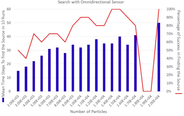
Figure1depicts some statistical information about the success rate for a group of three robots searching for the source of plume dispersion in a field of size 200×200 units. For each number of particles 10 experiments are done and for each experiment the probability field and the position of the robot is randomly initialized. The left axis indicates the mean time of finding the source of dispersion for each series of experiments. The criteria to find the source includes the mean distance of the particles from the source.
Figure 1.The bars plotted on the left axis indicate the mean number of timesteps to find a source in a 200×200 unit search field by a group of three robots. At each trial, the robots start from a predefined initial state chosen randomly beforehand. The initial position of the robots is constant for all the simulations, and the only difference is the hypotheses. The red plot displayed on the right axis shows the percentage of the time the team successfully located the source for 10 trials. By increasing the number of the particles the success rate increases. However, in none of the trials with 1.8×10⁴and 1.9×10⁴particles the robots were successful in finding the source. The overall results display a high uncertainty in the success of the mission to find the source.
A high number of the particles needed to perform the localization of the source also cause a serious problem in the implementation of the algorithm in a real world experiment. As we increase the number of particles the resolution of the grid map which covers the search field must also increase in order to accommodate them. However, the localization capability and control precision of the mobile robot sets a high bar for this resolution. Throughout this paper we have tried to use realistic measures for the simulations. For example, for all the simulations the field is assumed to be 200×200 units. This unit can be meter, and the size of the search field and the one-meter-grid-size are both sound realistic, but marginal. Any further increase in the number of particles might not be feasible from the robots’ capability point of view.
3.3.2. Value of Information
The results for the simulations of the simple collaborative search with a group of three robots does not show the expected improvement in the time and efficiency of the search. Surely, as more robots participate in the search the chance of registering a chemical patch will be higher. However, the simulations suggest that merely increasing the number of the explorers will not result in better performance. One of the reasons is the way we contribute the extracted information from the sensory events into the estimation of the probability field.
Detecting the presence of chemicals is a stochastic event and incorporating all the events happening to a multi-agent search group into the estimation of each agent participating in the search mission is misleading. For example, consider if one of the agents detects a fair number of cues—neglecting any error and with full faith on the sensors, eventually, it can estimate the position of the source of dispersion. On the other hand, if at the same time another agent does not receive any cue and incorporates the subsequent null events into the overall estimation process this will dilute the information gathered by the first agent.
a measure to decide which data can be informative and useful to be considered in the robots estimation, and which data received from other robots must be simply ignored. In this approach the value of the information which any event conveys is defined as the effect of event in the estimation of the probability distribution. This can be quantified as two factors:
1. how probable that event is, considering the current estimate the agent has; and,
2. how informative it is; this is measured with the information it carries, or in other words, the change it makes in the estimated probability field.
The probability of experiencing the reported event with an agent in the group can be calculated by (3) and (4). If the current probability field over the position of the source estimated with the Robot AisPA(r), then we can calculate the expected rate of positive sensor measurements and consequently the probability of such an event at the position of the robotBas:
hB= Z
PA(r)R(rB|r)dr → ρB=hBe−hB (13) Also, we can calculated how the probability field estimated with the RobotAwill change if it is certain that a positive sensor reading is happened at the position of the robotB. This is not different than the routine followed with a single robot in Algorithm1using (5).
Remark 3. We note that in our simulations, a robot does not always contribute its own positive sensor detection into the estimate of the source location. This is because while the probability of a positive detection event might be small by any robot in the team, if such an event changes the probability landscape considerably, it would be incorporated into the source position estimate. In this work, we assume perfect sensor readings and leave analyzing the effect of sensor noise and faults as a direction for future work.
4. Simulations
Figure2shows the trajectory of the robot searching for the source of dispersion located at the middle of the arena. The dimension of the arena is 200×200 units and the maximum speed of the robot is 2 units at each step. The observation model,R(r|r0)is only the function of distance of the robot from the hypothetical source location. As the robot moves through the environment the algorithm gradually eliminates particles. The number of the particles decreased dramatically after the first detection. After a few detections the particles concentrate on the estimated position of the source.
In the simulation results shown in Figure2it is assumed that the chemical dispersed from the source is propagated symmetrically by means of diffusion. Then, regardless of the direction it faces, the robot samples the medium and detects the presence of the chemical in the environment. In a more common scenario the robot is looking for the source of leakage where there is a background flow carrying the chemical through the environment. Moreover, the sensor on the robot can only detect the presence of the chemical as it enters the funnel leading to the sensor. To simulate such scenarios we assume the latest and do not change the behavior of the environment. The probability of registering the presence of a material patch by a sensor depends on the distance of the sensor from the source and angle between(r−r0)and the current course of robot immediately before it makes the observation,v:
R(r|r0) = R ln(λ
a)
e2VD(r−r0)·vK
0
|
r−r0|
λ
. (14)
the hypotheses in front of the robot are more likely to be the position of the source as compared to those behind.
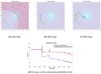
(a)20th Step (b)40th Step (c)80th Step
(d)Entropy of the estimated probability field.
Figure 2. (a–c) The trajectory for a single robot searching for a source of chemical dispersion and the variation (d) of the entropy of the estimated probability distribution. The red plot indicates the change in entropy the robot predicts upon the move, while the blue plot is the entropy of the estimation calculated after performing the observation. About 10,000 particles are initially generated to estimate the probability distribution. The size of the particles does not represent the associated weight of the particle.
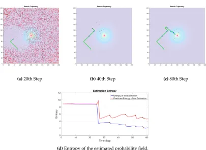
When the direction is involved in the estimation, as it can be seen from Figure3the consequent observations does not carry the amount of information they convey in the non-directional case. First detection conveys a lot of information on whereabouts of the source, as it can basically eliminate all the possibilities behind the robot. However, an immediate next detection of a cue might not be as informative as the first one as the robot is already confident that the source of the plume is not on its behind.
(a)20th Step (b)40th Step (c)80th Step
(d)Entropy of the estimated probability field.
Figure 3. (a–c) Search trajectory for a single robot searching for a source of chemical dispersion; (d) Variation of the entropy for the estimated probability distribution. The probability of detecting a chemical cue is proportional to the bearing of the robot with respect to the sources position. The chance of detecting a cue increases when the robot is moving toward the source. Red plot indicates the change in entropy the robot predicts upon the move, while the blue plot is the entropy of the estimation calculated after performing the observation. About 10,000 particles are initially generated to estimate the probability distribution. Size of the particles doesnotrepresent the associated weight of the particle.
(a)10th Step (b)20th Step (c)60th Step
(d)Entropy of the estimated probability field.
Figure 4. (a)–(c) Search trajectory for a single robot searching for a source of chemical dispersion; (d) Variation of the entropy for the estimated probability distribution. The motion model of the robot injects uncertainty on the position of the robot, and consequently on the hypothesis of the particles. The sensing capability of the robot is assumed to be independent of the bearing of the robot, then the uncertainty in direction of the robot is not included in the estimation process. Red plot indicates the change in entropy the robot predicts upon the move, while the blue plot is the entropy of the estimation calculated after performing the observation. About 3000 particles are initially generated to estimate the probability distribution. Size of the particles doesnotrepresent the associated weight of the particle.
Figure 5 depicts the simulation results of a robot searching for the source of a dispersion. The simulation results indicate that a manageable number of Gaussian like basis functions with well-tuned parameters can efficiently cover the search arena; the estimate efficiently converges to the position of the source as we incorporate new information using the proposed method.
(a)10th Step (b)20th Step
(c)40th Step (d)60th Step
(e)Entropy of the estimated probability field.
Figure 5.(a)–(d) The trajectory for a single robot searching for the source a of chemical dispersion. The probability field is spanned with 100 Gaussian functions each with a weight adjusted by each observation; (e) Variation of the entropy for the estimated probability distribution. The sensing capability of the robot is assumed to be independent of the bearing of the robot. The red plot indicates the predicted change in entropy for the next move while the blue plot is the actual entropy of the estimation after integrating the observation.
The same routine to update the estimate, shown in (3), (4), and (7), is applied to the weight of each Gaussian function, the main difference being the control algorithm design and waypoint selection procedure. In (5), the probability of finding the source at the very next step,ρ(r(t0)), is calculated from
the Gaussian mixture model used to estimate the probability field. Next, the predicted change in the probability field,∆Sis also calculated based on the same mixture model. The union of these functions directs the robot to the most probable position of the source in the search arena.
4.1. Multi-Robot Collaborative Search
Figure 6 shows the simulation results for a group of three robots. During the exploration, each negative sensor reading causes the weights of a large number of particles in the estimated probability field to be attenuated and subsequently eliminated during re-sampling. As a result of the extensive exploration performed before the detection, the first positive detection made by one of the robots causes a large number of the particles to be lost.
The communication between the agents is synchronized. With a constant frequency all the members of the search group share their sensory events. Every message package includes the sensor reading and the position and/or orientation (state) of the robot at the moment. As a result of the extensive exploration performed before the detection, the first positive detection made by one of the robots causes a large number of the particles to be lost. Intuitively, suppose a robot is moving in a direction for a while and is not detecting any cue. When the robot receives an information about another robot which has detected a cue moving in different direction, it will lose confidence on its estimations of the probable position of the source in front of it. This will show up in the mathematics of the problem with suddenly eliminating a large number of low probable hypothesis. The 20th step of the simulation in Figure6depicts this phenomena.
The probability distribution estimated by each robot is not exactly similar to their peers’ in the group. Beside the different initialization of each estimation, every robot also individually decides on the information it will involve in its estimated probability distribution. However, the simulations indicate that this algorithm results in similar estimations for all the members of the search group. The proof of this convergence will be the subject of further investigation, and does not fit to the scope of this paper.
(a)10th Step (b)20th Step (c)21th Step
(d)Entropy of the estimated probability field.
Figure 6. (a)–(c) The trajectory of a member of a group of three robots searching for the source of chemical dispersion. Each observation is communicated to the group and each member of the group use the information it gets from the others to manipulate its estimation. The green stars indicate the position where the other member of the group make a positive observation; (d) Variation of the entropy for the estimated probability distribution initially containing around 14,000 particles. Note that the size of the particles does not represent the associated weight of the particle.
(a)Agent 1: 10th Step (b)Agent 2: 10th Step (c)Agent 3: 10th Step
(d)Agent 1: 20th Step (e)Agent 2: 20th Step (f)Agent 3: 20th Step
Figure 7.Search trajectory for a group of three robots searching for a source of chemical dispersion. The sensing capability of the robot is assumed to be independent of the bearing of the robot, then the uncertainty in direction of the robots is not included in the estimation process. The probability field is spanned by 300 Gaussian functions, which in this pictures are shown by a particles. Size of the particles
doesrepresent the associated weight of the particle. Each robot builds a probability distribution over the position of the source individually. At each step of time, every robot propagates the event it experiences. The other robots calculate the value of information encapsulate in that event and decide whether or not they contribute that sensor event to its estimation. The probability distribution for the Agent 1 is pictured in 3D in Figure8.
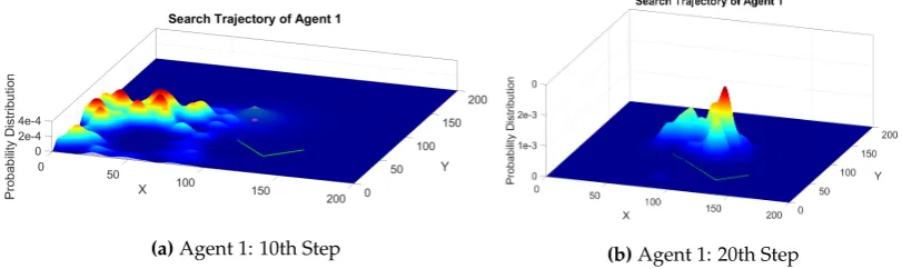
(a)Agent 1: 10th Step (b)Agent 1: 20th Step
Figure 8.3D probability distribution estimated over the possible positions of the dispersion source by the Agent 1. No particle is lost in the estimation process, and the incoming information stream is used to adjust the weights of the Gaussian functions.
4.2. Experimental Results
In this section we present an experiment based on the method presented in the previous sections. First, we examine the simulation results for a multi-robot team executing the described information theoretic strategies in 2D turbulent field; and then, The single-robot experiment based on the simulated plume is run with a mobile robot. The 2D dispersion model used in our simulations were developed to model the 2010 Deep Water Horizon Oil Spill. The dispersion database was obtained from a numerical simulation of a bubble plume in a stably stratified environment under rotation. The details and derivation of the turbulence resolving model for multiphase plumes are presented in [19]. Specifically, the plume is generated by an inlet buoyancy fluxBi=gwiAiαb,i =5×10⁻⁶m4s−3whereg=9.8 ms−2 is the gravity acceleration magnitude,wi=4 cm·s−1is the inlet liquid velocity,Ai =πr2i =0.005 m2is
the source cross-section area of radiusriandαb,i=0.026 is the inlet gas volume fraction. The initially unperturbed ambient fluid is thermally stratified with a constant slopeζ=5.1 K·m−1and the system
numerical sponges to ensure numerical stability. The domain has been spatially discretized using spectral element methods intoK=7540 conforming elements in which the solution is approximated with a 14th order polynomial expansion resulting in∼21 million nodes. The transport equations have been integrated using the nek5000 solver [28] that has demonstrated an excellent scalability on parallel machines [29]. The results used in this work correspond to the statistically stationary solution obtained after approximately 150,000 core-hours on a Cray XE6 using 960 2.2 GHz AMD Magny-Cours cores.
Figure9shows the search trajectories for a team of three robots. The dimensions of the simulation arena is 748×322 units, and the maximum reach of the robot at each time step is 5 units at each direction. The probability field is spanned by 100 Gaussian functions. At each step of time, every robot propagates the event it experiences. The other robots calculate the value of information encapsulated in that event and decide whether or not they incorporate the sensory event to its estimation (see Section3.3.2). The weights of these Gaussian functions are adjusted according to the procedure described in Section3.2. The sensor model for the robots is directional, however, the robots are free to move in any directions.
(a)20th Step (b)40th Step (c)80th Step
Figure 9.A group of three Robots searching for the source of chemical dispersion. The red dots indicates the positive sensor readings. The 2D dispersion model used in this simulations is developed to simulate the 2010 Deep Water Horizon Oil Spill. The dimensions of the simulation arena is 748×322 units, and the maximum reach of the robot at each time step is 5 units at each direction. The probability field is spanned by 100 Gaussian functions. At each step of time, every robot propagates the event it experiences. The other robots calculate the value of information encapsulate in that event and decide whether or not they contribute that sensor event to its estimation.
The Gaussian functions used to estimate the probability distribution function are spanned in three dimension, namelyXdirection andYdirection for the position of the robots, andθfor the heading
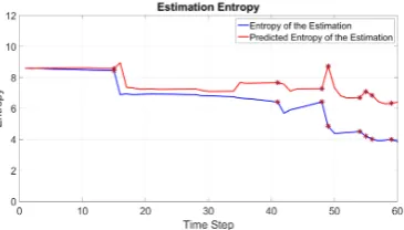
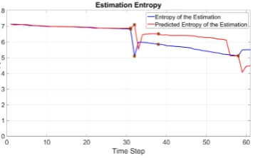
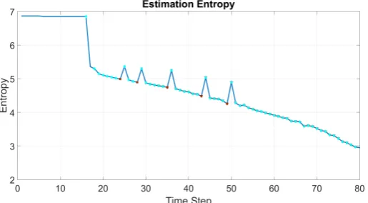
Figure 10.Variation of the entropy for the estimated probability distribution estimated by 100 weighted Gaussian functions. This entropy is related to the probability distribution estimated with one of the robots. The sensor detection with the robot is indicated with cyan diamonds, and the positive sensory events reported with other members of the team and contributed to the estimation is indicated with brown circles. As it can be seen these extra informations first disturbs the decreasing proceeding of the entropy of the estimation. However, eventually get in line with the general estimation of the robot.
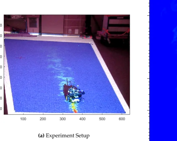
We examine the performance of the algorithm in a real experiment with a single mobile robot, and simulated plume which is projected on the search arena. Figure11a shows the experimental setup to search for the source of oil spill. The SAS Lab’s TIM robots is searching for the source of oil spill simulated to predict the behavior of the Deep Horizon, and projected on the ground. Measuring 20cm in diameter, these differential drive ground vehicles are equipped with an Odroid-U3+, running Ubuntu and ROS, an Asus Xtion Pro Live, and WiFi communication. Localization is provided by wheel odometry over short distances and by an overhead motion capture system covering the experimentation space, and transfered to the computer over the network. The Robot Operating System (ROS) environment is managing the data transfer and control of the robot; but, the main algorithm is implemented by Matlab software.
(a)Experiment Setup
(b)Robot’s Trajectory in Search for the Source
Figure 11.The experimental setup to search for the source of oil spill. The robot is searching for the source of oil spill simulated to predict the behavior of the 2010 spill in Deep Horizon. The position of the mobile robot is observed with motion capture cameras, and connected to the computer over the network. The Robot Operating System (ROS) environment is managing the data transfer and control of the robot. The algorithm is implemented by Matlab software.
5. Conclusions
of any information they receive from their peers in the group. The simulations shows the effectiveness of the method in such a realistic simulation.
Acknowledgments:This work was supported by the National Science Foundation (NSF) grant IIS- 1253917 and the Gulf of Mexico Research Initiative (GoMRI) Award No. SA 15-15.
Author Contributions:Main text.
Conflicts of Interest:‘The authors declare no conflict of interest.
References
1. Chang, D.; Wu, W.; Webster, D.R.; Weissburg, M.J.; Zhang, F. A bio-inspired plume tracking algorithm for mobile sensing swarms in turbulent flow. In Proceedings of the 2013 IEEE International Conference on Robotics and Automation (ICRA), 6–10 May 2013; pp. 921–926.
2. Vergassola, M.; Villermaux, E.; Shraiman, B.I. ‘Infotaxis’ as a strategy for searching without gradients.Nature
2007,445, 406–409.
3. Russell, R.A. Locating underground chemical sources by tracking chemical gradients in 3 dimensions. In Proceedings of the 2004 IEEE/RSJ International Conference on Intelligent Robots and Systems (IROS 2004), 28 September–2 October 2004; Volume 1, pp. 325–330.
4. Eisenbach, M.Chemotaxis; Imperial College Press: London, UK, 2004.
5. Kazadi, S.; Goodman, R.; Tsikata, D.; Green, D.; Lin, H. An autonomous water vapor plume tracking robot using passive resistive polymer sensors.Auton. Robots2000,9, 175–188.
6. Zhang, S.; Martinez, D.; Masson, J.B. Multi-robot searching with sparse cues and limited space perception.
Front. Robot. AI2015,2, 1–11.
7. Ferri, G.; Jakuba, M.V.; Mondini, A.; Mattoli, V.; Mazzolai, B.; Yoerger, D.R.; Dario, P. Mapping multiple gas/odor sources in an uncontrolled indoor environment using a Bayesian occupancy grid mapping based method.Robot. Auton. Syst.2011,59, 988–1000.
8. Wu, W.; Zhang, F. Robust Cooperative exploration with a switching strategy. IEEE Trans. Robot. 2012,
28, 828–839.
9. Hayes, A.T.; Martinoli, A.; Goodman, R.M. Distributed odor source localization. IEEE Sens. J.2002,
2, 260–271.
10. Zarzhitsky, D.V.; Spears, D.F.; Thayer, D.R. Experimental studies of swarm robotic chemical plume tracing using computational fluid dynamics simulations.Int. J. Intell. Comput. Cybern.2010,3, 631–671.
11. Stachniss, C.; Plagemann, C.; Lilienthal, A.J. Learning gas distribution models using sparse Gaussian process mixtures.Auton. Robots2009,26, 187–202.
12. Papoulis, A.; Pillai, S.U. Probability, random variables, and stochastic processes. InMcGraw-Hill Electrical and Electronic Engineering Series, 4th ed.; McGraw-Hill: New York, NY, USA, 2002.
13. Mesquita, A.R.; Hespanha, J.P.; Åström, K. Optimotaxis: A Stochastic Multi-agent Optimization Procedure with Point Measurements. In Proceedings of the 11th International Workshop on Hybrid Systems: Computation and Control, St. Louis, MO, USA, 22–24 April 2008; pp. 358–371.
14. Marjovi, A.; Marques, L. Multi-Robot Odor Distribution Mapping in Realistic Time-Variant Conditions. In Proceedings of the 2014 IEEE International Conference on Robotics and Automation (ICRA), 31 May–7 June 2014; pp. 3720–3727.
15. Hajieghrary, H.; Hsieh, M.A.; Schwartz, I.B. Multi-agent search for source localization in a turbulent medium.
Phys. Lett. A2016,380, 1698–1705.
16. Hajieghrary, H.; Tom, A.F.; Hsieh, M.A. An information theoretic source seeking strategy for plume tracking in 3D turbulent fields. In Proceedings of the 2015 IEEE International Symposium on Safety, Security, and Rescue Robotics (SSRR), West Lafayette, IN, USA, 8–20 October 2015; pp. 1–8.
17. Chirikjian, G.S. Information theory on Lie groups and mobile robotics applications. In Proceedings of the 2010 IEEE International Conference on Robotics and Automation (ICRA), 3–7 May 2010; Volume 10, pp. 2751–2757.
18. Charrow, B.; Michael, N.; Kumar, V. Cooperative multi-robot estimation and control for radio source localization.Springer Tracts Adv. Robot.2013,88, 337–351.
20. Hoffmann, G.M.; Tomlin, C.J. Mobile sensor network control using mutual information methods and particle filters.IEEE Trans. Autom. Control,2010,5, 32–47.
21. Charrow, B.; Liu, S.; Kumar, V.; Michael, N. Information-theoretic mapping using Cauchy-Schwarz Quadratic Mutual Information. In Proceedings of the IEEE International Conference on Robotics and Automation (ICRA), 26–30 May 2015, pp. 4791– 4798.
22. Thrun, S.; Burgard, W.; Fox, D.Probabilistic Robotics (Intelligent Robotics and Autonomous Agents); The MIT Press: Cambridge, MA, USA, 2005.
23. Schon, T.; Gustafsson, F.; Nordlund, P.-J. Marginalized particle filters for mixed linear/nonlinear state-space models.IEEE Trans. Signal Process.2005,53, 2279–2289.
24. Crisan, D.; Doucet, A. A survey of convergence results on particle filtering methods for practitioners.
IEEE Trans. Signal Process.2002,50, 736–746.
25. Gelman, A.; Carlin, J.B.; Stern, H.S.; Dunson, D.B.; Vehtari, A. Bayesian Data Analysis. InTexts in Statistical Science, 3rd ed.; CRC Press: Boca Raton, FL, USA, 2014.
26. Huber, M.F.; Bailey, T.; Durrant-Whyte, H.; Hanebeck, U.D. On entropy approximation for Gaussian mixture random vectors. In Proceedings of the IEEE International Conference on Multisensor Fusion and Integration for Intelligent Systems, 20–22 August 2008; pp. 181–188.
27. Howlett, R.J.; Jain, L.C. Radial Basis Function Networks 1: Recent Developments in Theory and Applications. InStudies in Fuzziness and Soft Computing; Physical-Verlag: Heidelberg, Germany, 2001.
28. Deville, M.O.; Fischer, P.F.; Mund, E.H. High-Order Methods for Incompressible Fluid Flow; Cambridge University Press: Cambridge, UK, 2002.
29. Fischer, P. F.; Lottes, J.W.; Kerkemeier, S.G. Nek5000 Web Page, 2008. Available online: http://nek5000.mcs. anl.gov.
30. https://www.youtube.com/playlist?list=PLmamVA9vIjfoP-5QyUlH7OW7KZhmzFYuF.
c