Abstract— Gene expression programming (GEP) is a data driven evolutionary technique that well suits for correlation mining. Parallel GEPs are proposed to speed up the evolution process using a cluster of computers or a computer with multiple CPU cores. However, the generation structure of chromosomes and the size of input data are two issues that tend to be neglected when speeding up GEP in evolution. To fill the research gap, this paper proposes three guiding principles to elaborate the computation nature of GEP in evolution based on an analysis of GEP schema theory. As a result, a novel data engineered GEP is developed which follows closely the generation structure of chromosomes in parallelization and considers the input data size in segmentation. Experimental results on two data sets with complementary features show that the data engineered GEP speeds up the evolution process significantly without loss of accuracy in data correlation mining. Based on the experimental tests, a computation model of the data engineered GEP is further developed to demonstrate its high scalability in dealing with potential big data using a large number of CPU cores.
Index Terms — Gene expression programming, schema theory, data engineering, big data analytics, parallelization and segmentation.
I. INTRODUCTION
ENE expression programming (GEP) [1] is a member of
Evolutionary Algorithms (EAs) [2] with a similar idea to both Genetic Algorithms (GAs) [3] and Genetic Programming (GP) [4]. GEP operates on a genotype-phenotype system to handle the representation of a candidate solution. GEP combines the linear structure of GA with the tree structure of GP providing a structured and flexible mechanism in searching for solutions.
GEP has been applied to many problems including combinatorial optimizations [6], finite transducers [42], classifications [7-10, 41], time series predictions [11-13] and symbolic regressions [14-16]. GEP was also employed to automatically generate a hyper-heuristic framework for combinatorial optimization problems [43, 44].
Zhengwen Huang, Maozhen Li and Ali Mousavi are with the Department of Electronic and Computer Engineering, Brunel University London, Uxbridge,
UB8 3PH, UK. Email: (zhengwen.huang, maozhen.li,
ali.mousavi)@brunel.ac.uk.
Maozhen Li is also associated with the Key Laboratory of Embedded Systems and Service Computing, Ministry of Education, Tongji University, Shanghai, 200092, China.
Christos Chousidis is with the School of Computing and Engineering, the
University of West London, W5 5RF, UK. Email:
Changjun Jiang is with the Department of Computer Science and Technology, Tongji University, 1239 Siping Road, Shanghai 200092, China. Email: cjjiang @tongji.edu.cn.
We have previously applied GEP in particle physics [17-19] to discriminate events from the background noisy signals. The performance was further improved with a prefix notation [20] to represent a candidate solution. In another work [39], we applied GEP to mine the correlations of Hadoop [40] parameters for big data analytics. GEP also has many applications in power systems such as the short-term load forecasting problem [21], and the static security problem [22].
The flexible structure of GEP together with its black-box style in solution searching makes GEP an appealing analytic approach to big data problems. However, the sheer size of big data would put a heavy burden on GEP computation in evolution. To speed up this process, a number of parallel GEP algorithms have been proposed using a cluster of computers [24, 26] or a single computer with multiple CPU cores [27]. Although the execution time of GEP decreases with an increasing number of CPU processors, these parallel GEPs suffer from two major limitations. On one hand, these parallel GEPs simply distribute the computation of chromosomes across a number of CPUs which breaks the generation structure of GEP leading to inefficiency in evolution. For example, the work presented in [26] assigns CPUs to process the chromosomes simultaneously, but it does not guarantee that the chromosomes of the same generation are assessed together in one iteration. On the other hand, these GEPs have not considered the size of an input data in parallelization leading to a scalability issue when dealing with an ever-growing size of potential big data. Therefore, the generation structure of chromosomes and the size of input data are two issues that tend to be neglected when speeding up the evolution process of GEP.
To fill the research gap, this paper presents a novel data engineered GEP and makes four major contributions:
• It proposes three guiding principles to elaborate the computation nature of GEP in evolution, which provides a theoretical foundation for GEP parallelization and segmentation. This is based on an analysis of our previous work on GEP schema theory [23] which is also highlighted by Zhong et al. in their work [38].
• Different from the existing GEP solutions, the data engineered GEP follows closely the generation structure of chromosomes leading to an efficient process in evolution.
• It employs two segmentation schemes to further speed up the evolution process. The cutting-in-sequence scheme segments an input data set into a number of overlapped data chunks with an aim to maintain the accuracy level of GEP in processing segmented data.
Schema Theory Based Data Engineering in Gene
Expression Programming for Big Data Analytics
Zhengwen Huang, Maozhen Li, Christos Chousidis, Ali Mousavi and Changjun Jiang
The random selection scheme selects samples from an input data set without overlapping and builds a single data chunk for processing.
• A computation model of the data engineered GEP is developed to demonstrate its high scalability in dealing with potential big data.
The data engineered GEP is evaluated on two data sets with complementary features. One data set has complex but loosely-coupled data samples in that each sample has a large number of input factors. The other data set has strongly correlated data samples but each sample has a small number of input factors. Experimental results show that the data engineered GEP reduces the computation time significantly without loss of accuracy in processing the segmented data chunks, which makes it scalable in dealing with potential big data problems.
The rest of this paper is organized as follows. Section II gives a review on related work. Section III proposes three guiding principles to elaborate the computation process of GEP based on an analysis of GEP schema theory. Section IV details the implementation of the data engineered GEP from the aspects of segmentation, overlapping and parallelization. Section V evaluates the performance of the data engineered GEP. Section VI develops a computation model to further demonstrate the scalability of the data engineered GEP in dealing with potential big data settings. Section VII concludes the paper and points out some future work.
II. RELATED WORK
The majority of existing works on data engineering in GEP only focus on parallelization. This section reviews some of the representative works in this aspect. It first reviews some works on schema theory which provides a theoretical foundation for GEP computation analysis.
A. Schema Theory
Schema theory is used to describe how EAs work under the pressure of selection. A solution provided by EAs can be considered as a point in a search space which contains all the possible solutions to a problem. The schemata of a chromosome containing such a solution can be considered as the coordinates of the point in the search space. In order to find the location of a good solution, a guided search space is provided by the schemata of a chromosome during the evolutionary process [3]. The schemata are generated by linking a set of schema elements based on the output of a fitness function. In this way, the search space containing a good solution is explored point by point in the search space and eventually the best solution can be generated.
Schema theory provides a theoretical support for analysis of EAs. By investigating the behaviors and the execution results of the genetic operations, the evolutionary process of EAs can be mathematically described with a set of formulas which are used to represent the propagation of schemata.
Holland developed a GA schema theory [3] to explain the evolutionary mechanism of GA. The theorem predicts the
number of strings matching a schema in the next generation based on the genetic information of the current generation. Following Holland’s GA schema theory, Koza [28] made the first attempt to define the schema in GP as a sub-space containing a set of sub-trees which share similar output behaviors. The GP schema is a tree structure which provides a deeper understanding of the input data. Poli and Langdon [30] introduced a fixed-size-and-shape schema which provides more restrictions on the shape of the S-expression program matching the schema. S-expression is a data representation of nested lists. In a later version, Poli and McPhee developed a Cartesian node reference system [31-32] to enhance the positional connection between the schema and the tree structure. Each position in the tree structure is indexed with one point in the node reference system. As a result, a more precise analysis of the propagation of the tree fragments matching the schema can be obtained. All these works try to provide a structured and flexible mechanism for a clear understanding of the GP evolutionary process.
GEP is a relatively new EA algorithm. As a result, few studies have been proposed on GEP schema theory. Cheng and Xue [29] attempted to define GEP schema following closely the work on GA schema theory. This work does not fully consider GEP specific features such as the head-tail structure of a chromosome, and the phenotype-genotype translation mechanism.
Huang [23] proposed a GEP schema theory which takes into account the GEP specific features in a systematic way. This work defines a schema together with a set of corresponding theorems to predict the propagation of a schema from one generation to another taking into account the head-tail structure of a chromosome. The phenotype-genotype separation is also considered. The genotype is used to select a schema which can be part of an entire chromosome, not only the part of the Open Reading Frame [1]. The phenotype is used only to provide the natural selection pressure through the fitness values of the chromosomes containing a schema.
Recently, Zhong et al. [38] proposed a self-learning GEP in which each chromosome is embedded with sub-functions that can be deployed to construct the final solution. It is worth noting that this work can be theoretically explained by the schema theory proposed in our previous work [23]. The evolutionary process is actually conducted by accumulating the genetic information on schemata which can be computed mathematically. As a result, the proposed self-learning GEP provides a mechanism to maintain the structure of the accumulated schemata which leads to an enhanced performance.
B. Parallel GEP
not significant especially when different types of CPU processors are used with varied computing powers.
The Asynchronous Distribute Parallel GEP based on the Estimation of Distribution Algorithm (ADPGEPEDA) further optimizes the load of each participating processor [26] using MPI. In ADPGEPEDA, each computer controls the evolutionary process of a part of the population independently. Since the computation capability of each participating computer is considered, ADPGEPEDA performs better than HPGEPSA in parallelization. However, the evolutionary process in ADPGEPEDA does not guarantee the chromosomes of the same generation would be assessed together in an evolutionary iteration which might break the nature of the selection process leading to an inefficient evolution.
Jiang et al. [27] presented a Parallel Niche GEP (PNGEPMP) using a single computer with multiple CPU cores for parallelization. Since there is no delay in computation among the homogeneous CPU processors, PNGEPMP achieves an impressive speedup in computation compared with ADPGEPEDA. However, PNGEPMP only focuses on covering more points in the search space by calculating the best fitness value generated from part of a chromosome, which does not represent the behavior of the whole chromosome. As a result, the accumulation of genetic information is not properly maintained in PNGEPMP.
Summarising, the aforementioned parallel implementations only focus on parallelization of the computation of GEP, but do not follow closely the generation nature of GEP leading to inefficiency in evolution. Furthermore, to make a parallel GEP scalable in dealing with potential big data, data engineering techniques such as segmentation should also be considered.
III. GEPSCHEMA AND COMPUTATION
In this section, we present three guiding principles to elaborate the computation nature of GEP. First we briefly describe how the genotype is translated into the phenotype in GEP and how the selection is conducted.
A. Genotype-Phenotype Translation
GEP combines a linear structured genotype chromosome with a phenotype Expression Tree (ET) [1] as shown in Fig.1. In this example the targeted problem has 4 input parameters (a, b, c, d) and 3 mathematic function operators { ′ + ′ , ′ − ′ , ′ ∗ ′ }. The chromosome has only one gene which is composed of a head and a tail. The elements of the head are selected randomly from both the input parameters and the mathematic function operators. The elements of the tail are selected randomly only from the input parameters.
The number of the elements of a gene is fixed which can be defined by user. The relation between the length of the head and the length of the tail can be calculated as
𝑇𝑎𝑖𝑙 = 𝐻𝑒𝑎𝑑 ∗ (𝑛— 1) + 1 (1)
where n is the maximum number of arguments that a
function operator requires.
The chromosome combines the input parameters and function operators during the evolutionary process. The ET is used to express the correlations among the input parameters. In this example, a candidate correlation among these parameters is represented with a combination of the function operators, i.e. ( a + b ∗ ( ( b – c ) ∗ a ) ). The translation from genotype to phenotype in GEP is conducted in the following steps:
(1) The element in the chromosome containing the function of
+ is selected to build the root of ET.
(2) The input parameter a and the function * are selected to be placed on Level_1 as the leaf nodes of the function of
+ in the ET.
(3) For the function of * in Level_1, another two elements (input parameter b and function *) are selected to be placed on Level_2 as the leaf nodes of the Level_1 function of * in the ET.
(4) The translation process continues until the ET is fully filled with the input parameters.
Fig.1. An example of translation from a chromosome to ET.
It is noted that not all the elements in the tail are involved in the translation process which is a typical feature of GEP (i.e. open reading frame [1]). Based on their fitness values, chromosomes in GEP are selected proportionally in evolving into the next generation.
B. GEP Computation Analysis
to the size of an input data set. The total execution time 𝑇 of a GEP evolutionary process can be calculated as
𝑇 = (𝑇𝑒×𝑇𝑑)×𝑁𝐺 (2) where
• 𝑇𝑒 is the time to go through the searchspacein one generation.
• 𝑇𝑑 is the time to process an input data set.
• 𝑁𝐺 is the number of generations.
The evolution of GEP is actually a process in which some segments of a chromosome are found useful and linked together to build the best chromosome. Considering the performance of the chromosomes that have similar genetic characteristics in the current generation, the schema theory [23] estimates the number of the chromosomes with such characteristics in the next generation. A schema is defined as a segment of a chromosome and maintains a certain amount of genetic information. In turn, a chromosome consists of a number of schemata representing all the possible solutions in a search space. The search space is created with the feature dimensions of an input data set and a chromosome which provides a structure to maintain the feature dimensions in the coordinate space.
The search space will be traversed during the evolutionary process to generate a number of schemata which are linked within a chromosome. The genetic information which is learned from the input data set is also accumulated by linking the schemata. At the end of the evolutionary process, the best chromosome which consists of the linked schemata is generated to represent the final solution to a targeted problem.
Based on the above analysis of the schema theory, we now propose three guiding principles to elaborate the computation nature of GEP evolution.
Guiding Principle 1: To efficiently accumulate the genetic information, the chromosomes of the same generation must be processed together in one evolutionary iteration.
Supporting Arguments: As indicated in the GEP schema theory, the evolutionary process is an accumulation of genetic information which is maintained in a chromosome. Schema is a segment of a chromosome which contains genetic information useful for a solution. The evolutionary process that a schema is propagated into the next generation can be represented by
𝐸[𝑀(𝐻, 𝑡 + 1)] = 𝑀×𝑃𝑅(𝐻, 𝑡)×𝑃𝐺𝑀(𝐻, 𝑡) (3)
where
• 𝐻 is a schema.
• 𝑡 is the number of generations.
• 𝑀 is the number of chromosomes in a generation.
• 𝑀(𝐻, 𝑡 + 1) is the number of chromosomes matching the schema 𝐻 in the generation of 𝑡 + 1.
• 𝐸[𝑀(𝐻, 𝑡 + 1)] is an estimation of 𝑀(𝐻, 𝑡 + 1).
• 𝑃𝑅(𝐻, 𝑡) is the probability of a chromosome that matches 𝐻 and is selected for Replication taking into
account all the chromosomes in the generation 𝑡.
• 𝑃𝐺𝑀(𝐻, 𝑡) is the probability that the schema 𝐻 is still
valid after the genetic modification process taking into account all the chromosomes in the generation 𝑡. • 𝑀×𝑃𝑅(𝐻, 𝑡)×𝑃𝐺𝑀(𝐻, 𝑡) is a theoretical number of
chromosomes matching the schema 𝐻 in the generation of 𝑡 + 1.
The evolution progresses with an increasing number of chromosomes that match the schema 𝐻 from one generation to the next generation. 𝑃𝑅(𝐻, 𝑡) relies on the genetic operations
which are performed on the chromosomes. A genetic operation is performed on all the chromosomes of the same generation with an aim to maximize the exchange of genetic information among these chromosomes. 𝑃𝑅(𝐻, 𝑡) can be calculated by
𝑃𝑅(𝐻, 𝑡) = 𝑀(𝐻, 𝑡)×𝑀×𝑓(𝑡)𝑓̅(𝐻,𝑡) (4)
where
• 𝑀(𝐻, 𝑡)is the number of the chromosomes matching H in the generation of 𝑡.
• 𝑓̅(𝐻, 𝑡) is the average fitness value of the chromosomes matching 𝐻 in the generation of 𝑡.
• 𝑓̅(𝑡) is the average fitness value of all the chromosomes in the generation of 𝑡.
Let 𝑃𝑅′(𝐻, 𝑡) represent the probability of a chromosome that matches 𝐻 and is selected for Replication taking into account only a group of the chromosomes in a generation. We have
𝑃𝑅′(𝐻, 𝑡) = ∑ (𝑃𝑅𝑖(𝐻, 𝑡)× 𝑚𝑖
𝑀) 𝑛
𝑖=1
= ∑ (𝑚𝑖(𝐻, 𝑡)×
𝑓̅𝑖(𝐻, 𝑡) 𝑚𝑖×𝑓𝑖(𝑡)
×𝑚𝑖 𝑀) 𝑛
𝑖=1
= ∑ (𝐹𝑖(𝐻, 𝑡) 𝐹𝑖(𝑡) ×
𝑚𝑖 𝑀) 𝑛
𝑖=1
≤ ∑𝐹𝑖(𝐻, 𝑡) 𝐹𝑖(𝑡) ×
𝑀 𝑀 𝑛
𝑖=1
= ∑𝐹𝑖(𝐻, 𝑡) 𝐹𝑖(𝑡) 𝑛
𝑖=1
≤ 𝑀(𝐻, 𝑡)×𝑓̅(𝐻, 𝑡) 𝑀×𝑓(𝑡)
(5)
where
• 𝑃𝑅𝑖(𝐻, 𝑡)is the probability of a chromosome matching 𝐻 that is selected from the 𝑖𝑡ℎ group of the chromosomes in the generation of 𝑡.
• 𝑛 is the number of groups of the chromosomes in the generation of 𝑡.
• 𝑚𝑖 is the number of chromosomes in the 𝑖𝑡ℎ group.
• 𝐹𝑖(𝐻, 𝑡) is the sum of the fitness values of the chromosomes matching 𝐻 in the 𝑖𝑡ℎ group of the generation of 𝑡.
• 𝐹𝑖(𝑡) is the sum of the fitness values of all the
Considering (4) and (5), we have
𝑃𝑅′(𝐻, 𝑡) ≤ 𝑃𝑅(𝐻, 𝑡) (6)
We denote 𝑃𝐺𝑀′(𝐻, 𝑡) as the probability that the schema 𝐻 is
still valid after the genetic modification process considering only a group of the chromosomes in a generation. Following the deduction process of (5), we have
𝑃𝐺𝑀′(𝐻, 𝑡) ≤ 𝑃𝐺𝑀(𝐻, 𝑡) (7)
Let 𝐸[𝑀(𝐻, 𝑡 + 1)]′ represent an estimation of the number of chromosomes that match the schema 𝐻 considering only a group of chromosomes in the generation of𝑡. Based on (6) and (7), we have
𝐸[𝑀[𝐻, 𝑡 + 1]] ≥ 𝐸[𝑀[𝐻, 𝑡 + 1]]′ (8)
which indicates that a group of chromosomes matching schema 𝐻 in a generation would lead to an evolutionary progress not faster than the case when all the chromosomes in the same generation are processed together.
Guiding Principle 2: A smaller size of an input data set leads to a faster evolutionary process of GEP.
Supporting Argument: The size of an input data set has an impact on the evolutionary progress of GEP. As indicated in (2), the time in processing an input data set (i.e. 𝑇𝑑) depends on the size of the input data which can be computed as
𝑇𝑑= ∑𝐺𝑗=1(∑𝑁𝑖=1𝑒(𝑇𝑒𝑖×𝑁𝑑))𝑗 (9) where
• 𝑁𝑒 is the number of elements in a chromosome.
• 𝐺 is the number of chromosomes in the current generation.
• 𝑇𝑒𝑖is the time needed to process the 𝑖𝑡ℎ element of a chromosome corresponding to a data point in the input data set.
• 𝑁𝑑 is the number of data points in the input data set. We denote 𝑇𝑑′ as the execution time to process a data chunk which is smaller than the original input data set. 𝑇𝑑′ can be computed as
𝑇𝑑′ = ∑𝐺𝑗=1(∑𝑁𝑖=1𝑒(𝑇𝑒𝑖×𝑁𝑑′ ))𝑗 (10)
where 𝑁𝑑′ is the number of data points in a data chunk. Based on (9) and (10), the execution time difference between the original input data set and a segmented data chunk can be computed as
𝑇𝑑− 𝑇𝑑′ = ∑ (∑(𝑇𝑒𝑖×𝑁𝑑)
𝑁𝑒
𝑖=1
)
𝑗 𝐺
𝑗=1
− ∑ (∑(𝑇𝑒𝑖×𝑁𝑑
′)
𝑁𝑒
𝑖=1
)
𝑗 𝐺
𝑗=1
= ∑ (∑ ((𝑇𝑒𝑖×𝑁𝑑)−(𝑇𝑒𝑖×𝑁𝑑′))
𝑁𝑒
𝑖=1
) 𝑗 𝐺
𝑗=1
=∑ (∑ (𝑇𝑒𝑖×(𝑁𝑑− 𝑁𝑑′ ))
𝑁𝑒
𝑖=1
)
𝑗 > 0 𝐺
𝑗=1
(11)
Guiding Principle 3: To achieve a fair selection of the chromosomes, an input data set must be segmented into equally sized chunks.
Supporting Argument: The evolutionary process
progresses with an increasing number of chromosomes matching the schema 𝐻 in each generation.
Let
• 𝐹 be the fitness function representing the performance of a chromosome in a generation.
• 𝑑𝑖 be the size of the 𝑖𝑡ℎ data chunk.
• 𝑐 be a chromosome.
• 𝑛 be the number of chromosomes matching a schema 𝐻.
• 𝐺 is the number of chromosomes in the current generation.
Considering (5), it can be observed that 𝑃𝑅(𝐻, 𝑡) depends on both 𝑓̅(𝐻, 𝑡) and 𝑓(𝑡) which can be computed by
𝑓̅(𝐻, 𝑡) =∑𝑛𝑖=0 𝐹(𝑐, 𝑑𝑖)
𝑛 (12)
𝑓(𝑡) =∑𝐺𝑖=0𝐹(𝑐, 𝑑𝑖)
𝐺 (13)
As a result, the probability that a chromosome is selected for evolution depends on the size of the data chunk that the chromosome processes. To ensure a fair selection, each chromosome is processed with data chunks of the same size which leads to an efficient evolution.
IV. DATA ENGINEERING IN GEP
Based on the proposed three guiding principles in Section III, we present a data engineered GEP to speed up computation in evolution.
A. Segmentation
select data samples from the original input data set and generate a data chunk. Each chromosome in a generation is processed with the same data chunk during the evolution of GEP. Cutting in sequence is implemented to cut the original input data set into a number of data chunks of an equal size in sequence.The order of the data samples in the data chunks remains the same as they appear in the original data set. While random selection targets at data samples without a strong correlation, the cutting in sequence segmentation scheme considers the correlations among the data samples of a data chunk.
B. Overlapping
While segmentation reduces the computation complexity of GEP, processing individual data chunks instead of the whole data set normally degrades the accuracy level of GEP [1]. This is especially true when the data samples have strong correlations. To minimize the accuracy degradation of GEP in data segmentation, an overlapping scheme is developed which takes into account the correlations among the data samples. Algorithm 1 presents the overlapping scheme implemented in the data engineered GEP.
Input: two data chunks (A, B) without overlapping; Output: two overlapped data chunks (A, B);
1: Set an overlapping ratio;
2: Calculate the number of samples to be overlapped; 3: FOR x=1 TO number of samples DO
4: Take a sample from the overlapped partition in data chunk A; 5: Overwrite the sample in the overlapped partition of data chunk B; 6: x++;
7: ENDFOR
8: RETURN data chunks A and B;
Algorithm 1: Overlapping implementation.
C. GEP Implementation
Considering segmentation and overlapping, the data engineered GEP is implemented as shown in Algorithm 2. The GEP takes an input data set, and generates a mathematical expression which represents the correlations of the input data parameters. The fitness evaluator of Line 9 assesses the performance of each chromosome in a generation following the classical fitness function proposed in [1]. This fitness evaluator has two versions, one is designed for the random selection segmentation scheme without overlapping, whereas the other is designed for the cutting in sequence segmentation scheme with overlapping. In the case of random selection, the quality of a chromosome is assessed considering the best local fitness value.
However, the assessment in the case of cutting in sequence follows the way as shown in Algorithm 3. In this case, the quality of a chromosome is assessed based on its global fitness value which is an average of the local fitness values of the chromosome when processing all the data chunks as shown in Lines 6-12. This helps prevent the GEP from trapping in a local optimum.
Input: A data set;
Output: A mathematical expression;
1: Segment the input data set into N data chunks 2: Generate N overlapped data chunks
3: Initialize the first generation of the population with more than N chromosomes;
4: best_chromosome = chromosome(1); 5: best_fitness_value = 0;
6: WHILE i< termination generation number DO
7: FOR x=1 TO size of the current population DO
8: Translate chromosome(x) into an expression tree(x);
9: global_fitness_value(x) =fitness_evaluator(expression_tree(x), N data_chunks);
10: IF global_fitness_value(x)=the number of samples in data_chunk(x) THEN
11: best_chromosome = chromosome(x) GOTO 21;
12: ELSE IF global_fitness_value(x) > best_fitness_value THEN
13: best_chromosome = chromosome(x); 14: best_fitness_value = global_fitness_value(x); 15: ENDIF
16: x++; 17: ENDFOR
18: Generate the population of the next generation; 19: i++;
20: ENDWHILE
21: RETURN best_chromosome;
Algorithm 2: GEP implementation.
Input: N data chunks and an expression_tree(x); Output: The fitness value of a given chromosome;
1: data_chunk_no = x mod N;
2: current_data_chunk = data_chunk(data_chunk_no);
3: local_fitness_value = fitness(expression(x), current_data_chunk); 4: fitness_value = local_fitness_value;
5: IF local_fitness_value > best_fitness_value THEN
6: FOR y=1 TO the number of N DO
7: current_data_chunk = data_chunk(y);
8: local_fitness_value=fitness(expression(x), current_data_chunk); 9: accumulation = accumulation + local_fitness_value; 10: ENDFOR
11: average_fitness_value = accumulation / N; 12: fitness_value = average_fitness_value; 13: ENDIF
14: RETURN fitness_value;
Algorithm 3: Fitness evaluator.
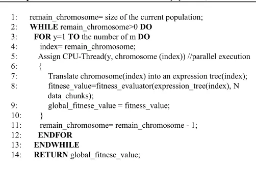
D. GEP Parallelization
Input:m CPU-threads, a population of chromosomes, N data chunks;
Output: the fitness values of chromosome in a population;
1: remain_chromosome= size of the current population; 2: WHILE remain_chromosome>0 DO
3: FOR y=1 TO the number of m DO 4: index= remain_chromosome;
5: Assign CPU-Thread(y, chromosome (index)) //parallel execution 6: {
7: Translate chromosome(index) into an expression tree(index); 8: fitnese_value=fitness_evaluator(expression_tree(index), N data_chunks);
9: global_fitnese_value = fitness_value; 10: }
11: remain_chromosome= remain_chromosome - 1; 12: ENDFOR
13: ENDWHILE
14: RETURN global_fitnese_value;
Algorithm 4: GEP parallelization.
V. PERFORMANCE EVALUATION
To evaluate the performance of the data engineered GEP, a number of experiments were conducted. This section analyzes the impact of segmentation, overlapping and parallelization on the performance of the GEP respectively. First it introduces the two data sets employed in the evaluation.
A. Data Sets
Two data sets were evaluated in the experimental tests which are detailed below.
Power system data set. The total data set contains 9568 data points (measurements) collected from a Combined Cycle Power Plant over 6 years [34, 35]. It consists of 5000 measurements for training and 4568 measurements for testing. Following our previous work presented in [39], GEP generates a mathematical function which represents the correlations of the power related environmental factors for production prediction of the power plant.
Particle physics data set. This data set [17, 18, 19] contains 10,000 samples of events of which the first 5000 samples were used for training and the rest were used for testing. A sample can be classified into an event signal or a background noise. Each sample has 8 input factors. Similar to the processing on the power system data set, the data engineered GEP also generates a mathematical function representing the correlations of the input factors which is used for classification.
It is worth noting that the use of two data sets in the evaluation has some considerations. On one hand, the time serial power system data set is not complex in that each data sample has a small number of factors with simple mathematical dependencies. However, the power data samples have a strong correlation among them. On the other hand, the particle physics data set is complex due to the large size of input factors of a data sample together with the mathematical or logical dependencies among these factors. Different from the power data set, the samples in the particle physics data set are not highly correlated. As a result, these two data sets with
complementary features were selected for evaluating the performance of the data engineered GEP.
B. GEP Parameter Settings
The settings of data engineered GEP are listed in Table 1. The parameters were set using the classical values used for a traditional GEP.
Table 1: GEP parameter settings.
Parameters Values
Population size 100 No. of genes in a chromosome
1
No. of generations Physics data 20000
Power system data 10000
Genetic modifications of
GEP
one-point recombination rate
30%
two-point recombination rate
30%
insertion sequence transposition rate
10%
inversion rate 10%
mutation rate 0.44%
One gene was employed for each chromosome to avoid the use of the connection function which might lead to an inefficient chromosome structure [1]. Considering the complexity of the two data sets, we set 20,000 generations for the physics data and 10,000 generations for the power data.
To evaluate the performance of the data engineered GEP, an Intel Xenon Server was configured with two Intel E5-2697 V2 CPU processors at 2.7GHz running Linux Ubuntu version 14.04. Each of the two processors has 12 CPU cores and supports 24 threads with a shared memory space of 64GB. We conducted 10 runs for each test in the evaluation and observed that the execution times of the 10 runs were highly stable. For example, Table 2 shows the coefficient of variation values of 9 tests on the two data sets which are in the range between 2.2% and 10.8%. As a result, an average value of 10 runs was taken for each test.
Table 2: Coefficient of variation values (%). Number of CPU
threads 1 2 3 4 8 12 16 24 48 Particle physics data 4.4 3.7 3.7 2.8 8.6 5.4 4.6 2.2 5.4 Power system data 10.8 10.5 8.3 9.6 8.8 7.8 6.2 6.9 8.3
C. Overlapping
A number of tests were conducted to evaluate the performance of the GEP with the cutting in sequence overlapping scheme from the aspects of both accuracy and execution time. Fig.2 and Fig.3 show the results of the GEP on the two data sets with a segmentation ratio of 10%.
the accuracy gain and execution time incurred. That was the reason why 50% was selected as the best overlapping ratio.
94.274 94.442 94.68 94.712 1534.86 1650.04 1854.65 2336.22
0 10 40 50 80
94.0 94.2 94.4 94.6 94.8 95.0
Overlap ratio (%)
A cc u ra cy ( % ) 1400 1600 1800 2000 2200 2400 Accuracy (%)
Execu tion time(s)
E xe c ut io n ti m e(s )
Fig.2. The impact of overlapping on particle physics data.
89. 652
97. 835
99. 057 99. 186
942.46
1061.08 1194.5
1720.06
0 1 0 4 0 5 0 8 0
8 8 9 0 9 2 9 4 9 6 9 8 1 00
Overlap rat io (%)
A ccu ra cy (% ) 6 00 8 00 1 00 0 1 20 0 1 40 0 1 60 0 1 80 0 2 00 0 Accuracy (%) Execution time(s) E xe cu tio n tim e( s)
Fig.3. The impact of overlapping on power system data.
D. Segmentation
The segmentation ratio determines the size of a data chunk that is assigned to each chromosome. Three segmentation ratios (i.e. 50%, 10% and 5%) were tested in the evaluation. Fig.4 shows the impacts of the segmentation ratios on the execution time of the data engineered GEP on the two data sets respectively.
Although the execution time of GEP decreases when the segmentation ratio goes down, a small segmentation ratio might lead to a low accuracy level in data processing. For example, when the segmentation ratio is 10%, the GEP produces an accuracy of 94.68% on the particle physics data and 99.06% on the power system data respectively. However, the case of using a segmentation ratio of 5% generates 93.942% on the particle physics data and 96.81% on the power system data in term of accuracy. As a result, a segmentation ratio of 10% was selected in the evaluation.
E. Parallelization
To evaluate the performance of the data engineered GEP in parallelization (denoted as P-GEP), we implemented an existing parallel GEP work (i.e. NICHE) [27] for comparison purpose. The number of CPU threads was varied from 1 to 48 in the tests. Two versions of the P-GEP were implemented. The P-GEP-overlap adopts the cutting in sequence segmentation scheme with overlapping whereas the P-GEP-random adopts the random segmentation scheme without overlapping.
5 10 50 100
0 2000 4000 6000 8000 10000 12000 14000 Execut ion time (s)
Segmentation ratio (%) Patical Physics Data Power System Data
Fig.4. The impact of segmentation on the two data sets.
It can be observed from Fig.5 and Fig.6 that the execution time of the P-GEP in processing both the particle physics data and the power system data decreases with an increasing number of CPU threads. The two versions of the P-GEP are significantly faster than the NICHE work. This is mainly due to the fact that P-GEP follows closely the generation structure of GEP leading to an efficient evolution. In addition, processing segmented data chunks further speeds up the computation. P-GEP-random is even faster than P-GEP-overlap because the less computation overhead incurred in accessing the multiple data chunks. It is worth noting that the execution time of the P-GEP in processing small data chunks does not decrease significantly when the number of CPU threads increases which reflects the fact that parallelization better suits big data processing which will be further discussed in Section VI.
1 2 3 4 8 12 16 24 48
0 2000 4000 6000 8000 10000 12000 14000 Exe cu tio n ti me (s)
Number of CPU threads
NICHE P-GEP_random P-GEP_overlap
Fig.5. The computation of the P-GEP on particle physics data.
1 2 3 4 8 12 16 24 48
0 1000 2000 3000 4000 5000 6000 7000 Execut ion time (s)
Number of CPU threads
NICHE P-GEP_random P-GEP_overlap
Fig.7 and Fig.8 show the accuracy of P-GEP in comparison with the NICHE work in processing the two data sets. The accuracy of P-GEP-overlap is similar to that of NICHE in all the tests. On average, P-GEP-overlap produces an accuracy of 94.57% on the particle physics data and 96.26% on the power system data whereas NICHE produces an accuracy of 94.62% and 94.83% respectively. It is worth noting that P-GEP-overlap is more accurate than P-GEP-random on the power system data due to the fact that overlapping well suits data sets such as the power system data with a strong correlation among data samples. The P-GEP-random produces the worst level of accuracy due to its random selection of data chunks without overlapping.
Fig.7. The accuracy of the P-GEP on particle physics data.
Fig.8. The accuracy of the P-GEP on power system data.
Fig.9 and Fig.10 further show that parallelization better suits for processing potential big data. It can be observed from Fig.9 that the execution time of P-GEP-overlap using a segmentation ratio of 50% decreases significantly when the number of CPU threads increases. However, P-GEP-overlap does not produce much difference in processing the particle physics data using a segmentation of 10% and 5% respectively. In the case of processing power system data as shown in Fig.10, the execution time of the parallel P-GEP-overlap using a segmentation ratio of 5% is even slower than the case of using a segmentation ratio of 10% when the numbers of CPU threads are 24 and 48 respectively. This is because the segmented power system data chunks are small in volume which leads to a higher overhead in parallelization than the speedup achieved in computation.
1 2 3 4 8 12 16 24 48
1000 2000 3000 4000 5000 6000
Execut
ion
time
(s)
Number of CPU threads
Partical_Physcis_Segmentation_Ratio (50%) Partical_Physcis_Segmentation_Ratio (10%) Partical_Physcis_Segmentation_Ratio (5%)
Fig.9. The impact of segmentation ratio on the execution time of
P-GEP-overlap in processing particle physics data.
1 2 3 4 8 12 16 24 48
500 1000 1500 2000 2500 3000 3500 4000
Execut
ion
time
(s)
Number of CPU threads
Power_System_Segmentation_Ratio (50%) Power_System_Segmentation_Ratio (10%) Power_System_Segmentation_Ratio (5%)
Fig.10. The impact of segmentation ratio on the execution time of the
P-GEP-overlap in processing power system data.
F. Statistical Analysis
To further compare the performance of the data engineered GEP with that of the NICHE work, we employed 48 CPU threads and conducted 50 runs in total on the two data sets respectively. The execution times in running the two algorithms follow a normal distribution as can be observed from Fig.11.
3100 3200 3300 3400 3500 3600 0
2 4 6 8 10 12 14 16 18 20 22 24
Cou
nts
NICHE execution time on physics data(s)
1400 1450 1500 1550 1600 1650 1700 1750 1800 1850 0
2 4 6 8 10 12 14 16 18 20
Coun
ts
NICHE execution time on power data(s)
300 350 400 450 500 550 600 650 700 750 0
2 4 6 8 10 12 14 16 18 20
Coun
ts
P-GEP execution time on physics data(s)
500 600 700 800 900 1000 1100 1200 1300 0
2 4 6 8 10 12 14 16 18 20
Coun
ts
P-GEP execution time on power data(s)
Fig.11. The distributions of the execution times of the P-GEP and
We further performed normality test on the execution times of the two algorithms using the Shaprio-Wilk test [46] which handles well with a small number of data samples. The W values of the Shaprio-Wilk tests as shown in Table 3 confirm the observed normal distributions as shown in Fig.11.
Table 3: The results of Shapiro-Wilk test.
Samples W values
NICHE (physics data) 0.920
NICHE (power data) 0.958
P-GEP (physics data) 0.988
P-GEP (power data) 0.957
Therefore, we employed t-test [45] to compare P-GEP with NICHE on the execution times which follow a normal distribution and the comparison results are shown in Table 4. It can be observed that the data engineered GEP with overlapping is faster than NICHE on both data sets at a significance level higher than 99.9%. We further observe that the accuracy of the data engineered GEP is slightly higher and more stable than that of NICHE. This is mainly due to the fact that the data engineered GEP considers the global fitness of chromosomes rather than their local values.
Table 4: The results of t-test.
Execution Time (s) Accuracy (%) mean t-value significance
level (%) mean deviation standard NICHE
(physics data) 3326.74
108.5 99.99
94.49 0.622 P-GEP (physics
data) 906.69 94.51 0.670
NICHE (power
data) 1625.99
4.506 99.99
96.65 8.685 P-GEP
(power data) 515.47 96.81 3.860
VI. GEPCOMPUTATION SCALABILITY ANALYSIS To further investigate the computation scalability of the data engineered GEP in dealing with potential big data using a large number of CPU threads, we developed its computation model based on the experimental results presented in Section V. In this section, we present the computation model and analyze the computation scalability of the data engineered GEP.
A. GEP Computation Model
Following our previous work [39] we developed a computation model of the data engineered GEP on the two data sets respectively, which represents the correlations between the input parameters (number of CPU threads 𝑥0, data size 𝑥1, segmentation ratio 𝑥2) and the output (execution time).
The computation model of the data engineered GEP for the particle physics data set can be represented by
𝐸𝑥𝑒𝑐𝑢𝑡𝑖𝑜𝑛𝑇𝑖𝑚𝑒 =
[−49.6019773651𝑆𝑖𝑛(𝑥
0) ∗ 𝑆𝑖𝑛(𝑥1)] + 2 ∗ ( 𝑆𝑞𝑢𝑎𝑟𝑒(𝑥0)
𝑆𝑞𝑟𝑡(𝑥1) ) + 𝑆𝑞𝑢𝑎𝑟𝑒(25.013766624)
+𝑆𝑞𝑟𝑡 (𝑃𝑜𝑤𝑒𝑟(20.9463112056,4)𝑆𝑞𝑟𝑡(𝑥
1) )
(14)
This is mined from the experimental results obtained using both 5% and 50% segmentation ratios on the physics data. These two ratios generated a large gap between the two result sets which leads to a highly accurate computation model in dealing with data samples with a large number of factors.
For the power system data, we employed the experimental results obtained using both 5% and 10% segmentation ratios to mine the computation model of data engineered GEP which can be represented by
𝐸𝑥𝑒𝑐𝑢𝑡𝑖𝑜𝑛𝑇𝑖𝑚𝑒 =
𝑃𝑜𝑤𝑒𝑟(𝑆𝑞𝑟𝑡(𝑥1− 𝑇𝐴𝑁(𝑥2)), 3) + ((𝑥0−𝑥1
𝑆𝑞𝑟𝑡(𝑥0)) ∗ (𝑥0− 𝑥2)) +
𝐶𝑜𝑠(𝐿𝑜𝑔(𝑥1)) ∗ (𝑆𝑞𝑢𝑎𝑟𝑒(𝑥0))+𝐶𝑜𝑠(𝑃𝑜𝑤𝑒𝑟(𝑥1, −401043.774094)) ∗
[𝑆𝑞𝑢𝑎𝑟𝑒(𝑥0)] − (𝑇𝑎𝑛 (𝐿𝑜𝑔 [𝑆𝑞𝑢𝑎𝑟𝑒 (80595.3126401𝑥1 )])
+𝑆𝑞𝑢𝑎𝑟𝑒(𝐿𝑜𝑔(𝑆𝑞𝑢𝑎𝑟𝑒 [−409114.183858
𝑥1 ])
+𝑆𝑞𝑢𝑎𝑟𝑒 (𝐿𝑜𝑔 (𝑆𝑞𝑢𝑎𝑟𝑒 [−22415.3897725 𝑥1 ])) ∗
𝑥2
100∗ 𝑥0
80.6 ∗ (𝑃𝑜𝑤𝑒𝑟 (1 + 0.6 ∗1
𝑥0, 𝑥0− 1) − 𝑃𝑜𝑤𝑒𝑟(1.0093, 𝑥0))
(15) The use of these two ratios on the power system data with a small gap aimed to reflect the fine-grained behaviors of the computation model in dealing with data samples with a small number of factors.
B. Validation of GEP Computation Model
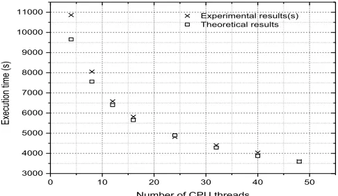
We employed the two data sets of the original sizes to generate the computation model to estimate the execution times of the data engineered GEP running on a varied number of CPU threads. To validate the computation model of the data engineered GEP, we compared the estimated values with the actual execution times in processing the two data sets but with doubled sizes. Fig.12 and Fig.13 show the performance of the computation model on the two data sets respectively using a segmentation ratio of 50%.
0 10 20 30 40 50
3000 4000 5000 6000 7000 8000 9000 10000 11000
Executio
n t
ime
(s)
Number of CPU threads
Experimental results(s) Theoretical results
0 10 20 30 40 50 1500
2000 2500 3000 3500 4000 4500 5000 5500
Execut
ion
time
(s)
Number of CPU threads
Experimental results Theoretical results
Fig.13. Computation model validation on power system data.
The accuracy of the computation model can be computed by
Accuracy =100% − (|𝑇ℎ𝑒𝑜𝑟𝑒𝑡𝑖𝑐𝑎𝑙 𝑅𝑒𝑠𝑢𝑙𝑡−𝐸𝑥𝑝𝑒𝑟𝑖𝑚𝑒𝑛𝑡𝑎𝑙 𝑅𝑒𝑠𝑢𝑙𝑡|𝐸𝑥𝑝𝑒𝑟𝑖𝑚𝑒𝑛𝑡𝑎𝑙 𝑅𝑒𝑠𝑢𝑙𝑡 ) ×100% (16) Table 4 and Table 5 show that the computation model achieves an average accuracy level of 96.05% on the particle physics data and 95.14% on the power system data respectively. Table 4. Computation model validation on particle physics data.
Number
of threads 4 8 12 16 24 32 40 48 Accuracy
level (%) 88.88 93.87 97.17 97.12 98.41 97.46 95.80 99.66 Average
(%) 96.05
Table 5. Computation model validation on power system data. Number
of threads 4 8 12 16 24 32 40 48 Accuracy
level (%) 99.40 91.84 91.93 93.44 94.02 98.42 94.31 94.78
Average
(%) 95.14
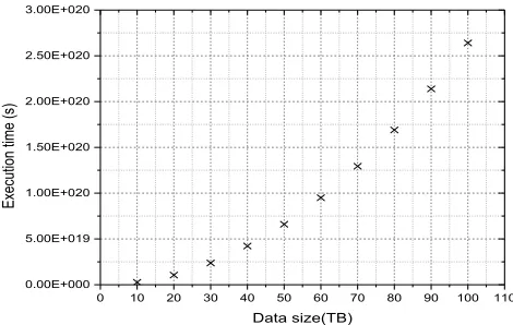
C. Computation Scalability
We applied the computation model to evaluate the scalability of the data engineered GEP in dealing with big data scenarios. Fig.14 and Fig.15 show that for the two data sets, the execution time of the data engineered GEP increases slowly with an increasing size of input data up to 100TB, using 10,000 CPU threads.
0 10 20 30 40 50 60 70 80 90 100 110 0.00E+000
1.00E+020 2.00E+020 3.00E+020 4.00E+020 5.00E+020 6.00E+020 7.00E+020 8.00E+020 9.00E+020 1.00E+021
Executio
n t
ime
(s)
Data size (TB)
Fig.14. Computation scalability on particle physics data.
0 10 20 30 40 50 60 70 80 90 100 110
0.00E+000 5.00E+019 1.00E+020 1.50E+020 2.00E+020 2.50E+020 3.00E+020
Executio
n t
ime
(s)
Data size(TB)
Fig.15. Computation scalability on power system data.
We further evaluated the computation scalability of the data engineered GEP in dealing with varied numbers of CPU threads. Fig.16 shows that the execution time of the data engineered GEP decrease when processing 1TB particle physics data with an increasing number of CPU threads up to 1000. It can be observed that the speedup of parallelization is high when the number of CPUs is less than 100 due to the fact that CPU threads themselves can also cause an additional computation overhead.
0 100 200 300 400 500 600 700 800 900 1000 1100 0.00E+000
1.50E+014 3.00E+014 4.50E+014 6.00E+014 7.50E+014 9.00E+014
Execut
ion
time
(s)
Number of CPU threads
Fig.16. Parallelization on particle physics data.
further observed in Fig.18 where a segmentation ratio of 5% was used on the two original data sets.
0 100 200 300 400 500 600 700 800 900 1000 1100 0.00E+000
2.00E+017 4.00E+017 6.00E+017 8.00E+017 1.00E+018 1.20E+018 1.40E+018 1.60E+018 1.80E+018 2.00E+018 2.20E+018 2.40E+018
Execut
ion
time
(s)
Number of threads
Fig.17. Parallelization on power system data.
0 20 40 60 80 100 120 140 160
300 400 500 600 700 800 900 1000 1100 1200
Execut
ion
time
(s)
Number of CPU Threads
Particle physics data set Power system data set
Fig.18. Fluctuations in performance gain via parallelization.
Overall the data engineered GEP achieves a high scalability in dealing with potential big data using a large number of CPU threads.
VII. CONCLUSION AND FUTURE WORK
In this research, we have presented an efficient data engineered GEP solution in dealing with potential big data. It builds on the proposed three guiding principles which necessitate the considerations on the generation structure of chromosomes, the size of input data and the segmentation of data chunks when speeding up the evolution process of GEP. Experimental results confirmed that the data engineered GEP which follows closely the generation structure of chromosomes in evolution and considers the size of input data did speed up the evolution process significantly without loss of accuracy in data correlation mining. The computation model further showed that the data engineered GEP is highly scalable in dealing with potential big data.
It should be pointed out that for data sets with a high volume in size but a low complexity in data structure, purely increasing the number of CPU threads could lead to slow executions due to the fact that the overhead incurred in maintaining these CPU threads is higher than the performance gain to be achieved through parallelization.
The data engineered GEP can further benefit from the schema theory proposed in our previous work [23] which
introduces the concept of building blocks in GEP evolution. A GEP building block is a segment shared by high quality chromosomes in a population which can be discovered during the evolutionary process. Building blocks can be used to replace the corresponding segments of low quality chromosomes for computation speedup in evolution. Therefore, a future work will research how the data engineered GEP can be integrated with building blocks.
A
CKNOWLEDGEMENTThis research is partially supported by the National Basic Research Program (973) of China under grant 2014CB340404, and also the Science and Technology Commission of Shanghai Municipality under grant 16JC1401300.
REFERENCES
[1] C. Ferreira, “Gene Expression Programming: a New Adaptive
Algorithm for Solving Problems”, Complex Systems, vol.13, no.2, pp.22, 2001.
[2] T. Bäck, Evolutionary Algorithms in Theory and Practice: Evolution Strategies, Evolutionary Programming, Genetic
Algorithms, 1996.
[3] JH. Holland, Adaptation in Natural and Artificial Systems: An Introductory Analysis with Applications to Biology, Control, and
Artificial Intelligence, U Michigan Press, 1975.
[4] J. R. Koza, “Genetic Programming as a Means for Programming
Computers by Natural Selection”, Stat. Comput., vol. 4, no. 2, pp. 87–112, 1994.
[5] D. H. Wolpert and W. G. Macready, “No Free Lunch Theorems for Optimization,” IEEE Trans. Evolutionary Computation, vol. 1, no. 1, pp. 67–82, 1997.
[6] C. Ferreira, “Combinatorial Optimization by Gene Expression Programming: Inversion Revisited,” in Proc. Argentine Symp. Artif. Intell., pp. 160–174, 2002.
[7] C. Ferreira, “Discovery of the Boolean Functions to the Best
Density-Classification Rules Using Gene Expression
Programming,” Genetic Programming, in Proc. of the 5th
European Conference, EuroGP 2002, vol. 2278, pp. 50–59, 2002.
[8] C. Zhou, P. C. Nelson, W.Xiao, & T. M. Tirpak, “Discovery of
classification rules by Using Gene Expression Programming,” in
Proc. of the Int. Conf. on Artificial Intelligence, pp. 1355-1361,
June, 2002.
[9] C. Zhou, W. Xiao, T. M. Tirpak, and P. C. Nelson, “Evolving
Accurate and Compact Classification Rules with Gene Expression Programming,” IEEE Transactions on Evolutionary
Computation, vol. 7, no. 6, pp. 519–531, 2003.
[10]M. H. Marghny and I. E. El-Semman. “Extracting Logical Classification Rules with Gene Expression Programming: Microarray Case Study,” in Proc. of the International Conference on Artificial Intelligence and Machine Learning (AIML 05),
Cairo, Egypt, 2005.
[11]J. Zuo, C. Tang, C. Li, C. Yuan, and A. Chen, “Time Series Prediction Based on Gene Expression Programming,” in Proc. of
the 5th International Conference on Advances in Web-Age
Information Management, WAIM 2004, vol. 3129, pp. 55–64,
2004.
[12]V. I. Litvinenko, P. I. Bidyuk, J. N. Bardachov, V. G. Sherstjuk,
and A. A. Fefelov, “Combining Clonal Selection Algorithm and Gene Expression Programming for Time Series Prediction,” in
Proc. of the Third Workshop IEEE Intelligent Data Acquisition
and Advanced Computing Systems: Technology and Applications,
[13]H. S. Lopes and W. R. Weinert, “A Gene Expression Programming System for Time Series Modeling”, in Proc. of XXV Iberian Latin American congress on computational methods
in engineering (CILAMCE), Recife, 2004.
[14]H. S. Lopes and W. R. Weinert, “An Enhanced Gene Expression Programming Approach for Symbolic Regression Problems,” Int.
J. Appl. Math. Comput. Sci., vol. 14, no. 3, pp. 375–384, 2004.
[15]Z. Cai, et al. “Symbolic Regression based on GEP and its Application in Predicting Amount of Gas Emitted from Coal Face,” in Proc. of the international symposium on safety science
and technology, 2004.
[16]E. Bautu, A. Bautu, and H. Luchian, “Symbolic Regression on
Noisy Data with Genetic and Gene Expression Programming,” in
Proc. of the Seventh International Symposium on Symbolic and
Numeric Algorithms for Scientific Computing (SYNASC’05), pp. 321–324, 2005.
[17]L. Teodorescu, and Z. Huang, “Enhanced Gene Expression
Programming for Signal-Background Discrimination in Particle Physics,” in Proc. of theXII Advanced Computing and Analysis
Techniques in Physics Research,2008.
[18]L. Teodorescu, “Gene Expression Programming Approach to Event Selection in High Energy Physics,” IEEE Transactions on
Nuclear Science, vol. 53, no. 4, pp. 2221–2227, 2006.
[19]L. Teodorescu, “High Energy Physics Data Analysis with Gene Expression Programming,” in Proc. of IEEE Nuclear Science
Symposium Conference Record, vol. 1, pp. 143–147, 2005.
[20]X. Li, C. Zhou, W. Xiao, and P. C. Nelson, “Prefix Gene Expression Programming,” in Proc. ofGenetic and Evolutionary
Computation Conference (GECCO), 2005.
[21]H. Limin, Y. Jinliang, G. Lirui, and H. U. Jie, “Short-Term Load Forecasting Based on Improved Gene Expression Programming,”
in Proc. of IEEE International Conference on Circuits and
Systems for Communications, 2008.
[22]S. F. Mekhamer, et al. “Gene Expression Programming for Power System Static Security Assessment,” International Journal of
Engineering, Science and Technology, vol.4, no. 2, pp.77-88,
2012.
[23]Z. Huang, “Schema Theory for Gene Expression Programming,”
PhD Thesis, Brunel University London, 2014.
[24]Z. Cai, et al, “A Novel Algorithm of Gene Expression Programming based on Simulated Annealing,” in Proc. of the International Symposium on Intelligence Computation &
Applications, vol. 610, 2005.
[25]M. Snir, S. Otto, S. Huss-Lederman, D. W. Walker, and J. Dongarra, MPI: The Complete Reference, vol. 2. 1996.
[26]X. Du, L. Ding, and L. Jia, “Asynchronous Distributed Parallel
Gene Expression Programming Based on Estimation of
Distribution Algorithm,” in Proc. of the 4th International
Conference on Natural Computation, pp. 433–437, 2008.
[27]W. Jiang, T. Li, B. Fang, Y. Jiang, Z. Li, and Y. Liu, “Parallel Niche Gene Expression Programming based on General Multi-Core Processor,” in Proc. of the International Conference on
Artificial Intelligence and Computational Intelligence (AICI),
vol.3, pp.75-79. 2010.
[28]J. R. Koza, “Genetic Programming as a Means for Programming Computers by Natural Selection,” Stat. Comput., vol. 4, no. 2, pp. 87–112, 1994.
[29]H. Cheng and J. Xue. “The Research on Evolution Schema Theorem on Gene Expression Programming,” in (Eds.) E. Mao, L. Xu and W. Tian, Emerging Computation and Information
technologies for Education, Springer Berlin Heidelberg, pp.
399-406, 2012.
[30]R. Poli and W. B. Langdon, “Schema Theory for Genetic Programming with One-Point Crossover and Point Mutation,”
Evolutionary Computation., vol. 6, no. 3, pp. 231–252, 1998.
[31]R. Poli and N. F. McPhee, “General Schema Theory for Genetic Programming with Subtree-Swapping Crossover: Part I,”
Evolutionary Computation vol. 11, no. 1, pp. 53-66, 2003.
[32]R. Poli and N. F. McPhee, “General Schema Theory for Genetic Programming with Subtree-Swapping Crossover: Part II”
Evolutionary Computation, vol. 11, no. 2, pp. 169-206, 2003.
[33]J. S. Vitter, “An Efficient Algorithm for Sequential Random Sampling,” ACM Transactions on Mathematical Software, vol. 13. pp. 58–67, 1987.
[34]P. Tüfekci, “Prediction of Full Load Electrical Power Output of a Base Load Operated Combined Cycle Power Plant using Machine Learning Methods,” Int. J. Electr. Power Energy Syst., vol. 60, pp. 126–140, 2014.
[35]H. Kaya, P. Tüfekci, and S. F. Gürgen, “Local and Global
Learning Methods for Predicting Power of a Combined Gas &
Steam Turbine,” in Proc. of the International Conference on Emerging Trends in Computer and Electronics Engineering
(ICETCEE), pp. 13–18, 2012.
[36]D. Novillo, “OpenMP and Automatic Parallelization in GCC,” in
Proc. of the GCC Developers Summit, 2006.
[37]R. Chandra, L. Dagum, D. Kohr, D. Maydan, J. McDonald, and R. Menon, Parallel Programming in OpenMP, vol. 129, 2001. [38]J. Zhong, Y. S. Ong and W. Cai, “Self-learning Gene Expression
Programming,” IEEE Transactions on Evolutionary
Computation, vol. 20, no.1, pp.65-80, 2016.
[39]M. Khan, Z. Huang, M. Li, G. A. Taylor and M. Khan,
“Optimizing Hadoop Parameter Settings with Gene Expression Programming Guided PSO”, Concurrency and Computation: Practice and Experience, DOI:10.1002/cpe.3786, 2016.
[40]Apache Hadoop, Available: https://hadoop.apache.org/. [Accessed: 28-June-2016].
[41]Stewart W. Wilson “Classifier Conditions Using Gene Expression Programming”, Lecture Notes in Computer Science
Volume 4998, pp 206-217, 2008.
[42]J.S. Manognya and L. P. Wang, “Gene Expression Programming for Induction of Finite Transducer”, in Proc. Of the 7th
International Conference on Information, Communications and
Signal Processing (ICICS 2009), pp. 1-5, 2009.
[43]N. R. Sabar, M. Ayob, G. Kendall and R. Qu, “A Dynamic
Multiarmed Bandit-Gene Expression Programming
Hyper-Heuristic for Combinatorial Optimization Problems,” IEEE
Transactions on Cybernetics, vol.45, no.2, pp. 217-228, 2015.
[44]N. R. Sabar, M. Ayob, G. Kendall and R. Qu, “The Automatic
Design of Hyper-Heuristic Framework with Gene Expression Programming for Combinatorial Optimization problems,” IEEE
Transactions on Evolutionary Computation, vol.19, no.3, pp.
309-325, 2015.
[45]J. F. Box, “Guinness, Gosset, Fisher, and Small Samples”,
Statistical Science, vol.2, no.1, pp. 45–52, 1987.
Zhengwen Huang received the Ph.D. degree from the Department of Electronic and Computer Engineering at Brunel University London, UK in July 2014. His research is focused on evolutionary algorithms (gene expression programming, genetic programming) and data engineering. He received the MSc degree from King's College London and his BSc from University of Science and Technology, China.
Maozhen Li is currently a Professor in the Department of Electronic and Computer Engineering at Brunel University London, UK. He received the Ph.D. degree from Institute of Software, Chinese Academy of Sciences in 1997. He was a Post-Doctoral Research Fellow in the School of Computer Science and Informatics, Cardiff University, UK in 1999-2002. His research interests are in the areas of high performance computing, big data analytics and intelligent systems. He is on the Editorial Boards of a number of journals. He has over 150 research publications in these areas. He is a Fellow of the British Computer Society.
Christos Chousidis received the Ph.D. degree from Department of Electronic and Computer Engineering at Brunel University London in 2013. He is currently a Senior Lecturer in Applied Sound Engineering in the School of Computing and Engineering at the University of West London, UK. His research is on data engineering with a special focus on audio wireless networks. He is a member of the Audio Engineering Society.
Alireza Mousavi received the Ph.D. degree from the Department of Electronic and Computer Engineering, Brunel University London, UK in 1998. He is a Reader of Systems Engineering and Computing. His research interest is in smart supervisory control and data acquisition systems applied to real-time systems modeling and optimization. The key areas of application are in stochastic modeling, ontology alignment and sensor networks. He is a member of the Institute of Engineering and Technology (IET).
Changjun Jiang received the Ph.D. degree from the Institute of Automation, Chinese Academy of Sciences, Beijing, China, in 1995. He was a Post-Doctoral Research Fellow at the Institute of Computing Technology, Chinese Academy of Sciences in 1997. Currently, he is a Professor with the Department of Computer Science and Engineering, Tongji University, Shanghai. He is also a council member of China Automation Federation and Artificial Intelligence Federation, the director of Professional Committee of Petri Net of China Computer Federation, and the vice director of Professional Committee of Management Systems of China Automation Federation. He was a visiting professor of Institute of Computing Technology, Chinese Academy of Science; a research fellow of the City University of Hong Kong, Kowloon, Hong Kong; and an information area specialist of Shanghai Municipal Government. His current areas of research are concurrent theory, Petri net, and