Efficient Characterization of Transmitter Output Jitter Components in 100GBASE-CR4 Ethernet

(1)

University of New Hampshire University of New Hampshire

University of New Hampshire Scholars' Repository

Master's Theses and Capstones Student Scholarship

Winter 2019

Efficient Characterization of Transmitter Output Jitter

Components in 100GBASE-CR4 Ethernet

Paul Alan Willis

University of New Hampshire, Durham

Follow this and additional works at: https://scholars.unh.edu/thesis

Recommended Citation Recommended Citation

Willis, Paul Alan, "Efficient Characterization of Transmitter Output Jitter Components in 100GBASE-CR4 Ethernet" (2019). Master's Theses and Capstones. 1334.

https://scholars.unh.edu/thesis/1334

This Thesis is brought to you for free and open access by the Student Scholarship at University of New Hampshire Scholars' Repository. It has been accepted for inclusion in Master's Theses and Capstones by an authorized administrator of University of New Hampshire Scholars' Repository. For more information, please contact

(2)

EFFICIENT CHARACTERIZATION OF TRANSMITTER OUTPUT JITTER COMPONENTS IN 100GBASE-CR4 ETHERNET

BY

PAUL WILLIS

BS, Electrical Engineering, University of New Hampshire, USA, 2015

THESIS

Submitted to the University of New Hampshire in Partial Fulfillment of

the Requirements for the Degree of

Master of Science in

Electrical and Computer Engineering

(3)

(4)

This thesis has been examined and approved in partial fulfillment of the requirements for the degree of Master of Science in Electrical and Computer Engineering by:

Thesis Director, Michael J. Carter, PhD. Associate Professor of Electrical Engineering

Nicholas J. Kirsch, PhD.

Associate Professor of Electrical Engineering

Richard A. Messner, PhD.

Associate Professor of Electrical Engineering

on 8/20/2019.

(5)

(6)

ACKNOWLEDGMENTS

(7)

NOMENCLATURE

Math functions

erf Gaussian error function

erf c Complementary error function

erf c−1 Inverse complementary error function

Symbols

δ−δ dual-Dirac

f0 −3 dBfrequency

Specifications

IEEE 802.3 Ethernet

IEEE 802.3 Clause 83D Electrical characteristics of CAUI-4,

100 Gb/s Ethernet across four lanes over chip-to-chip channel IEEE 802.3 Clause 92 Electrical characteristics of 100GBASE-CR4,

100 Gb/s Ethernet across four lanes over copper cable channel IEEE 802.3 Clause 93 Electrical characteristics of 100GBASE-KR4,

100 Gb/s Ethernet across four lanes over backplane channel IEEE 802.3 Clause 110 Electrical characteristics of 25GBASE-CR and 25GBASE-CR-S,

25 Gb/s Ethernet across a single lane over copper cable channel IEEE 802.3 Clause 111 Electrical characteristics of 25GBASE-KR and 25GBASE-KR-S,

25 Gb/s Ethernet across a single lane over backplane channel IEEE 802.3 Clause 120B.3 Electrical characteristics of 200GAUI-8 and 400GAUI-16,

200 Gb/s Ethernet across eight lanes and 400 Gb/s Ethernet across sixteen lanes over chip-to-chip channel

Abbreviations

BER Bit error rate

BERT Bit error rate tester

(10)

CDF Cumulative distribution function CDR Clock and data recovery

COM Channel Operating Margin DCD Duty-cycle distortion DDJ Data dependent jitter DJ Deterministic jitter DUT Device under test

EBUJ Estimated bounded uncorrelated jitter ECC Error correction code

EOJ Even-odd jitter

ERJ Estimated random jitter

ET Equivalent time

ETUJ Estimated total uncorrelated jitter

IEEE Institute of Electrical and Electronics Engineers ISI Intersymbol interference

JTF Jitter transfer function NRZ Non-return-to-zero

OJTF Observed jitter transfer function PAM Pulse amplitude modulation PDF Probability density function

PJ Periodic jitter

PLL Phase-locked loop

PRBS Pseudo random binary sequence

RJ Random jitter

RT Real time

RV Random variable

(11)

TIE Time interval error

TJ Total jitter

TOJ Transmitter output jitter

UI Unit interval

(12)

LIST OF TABLES

Table Page

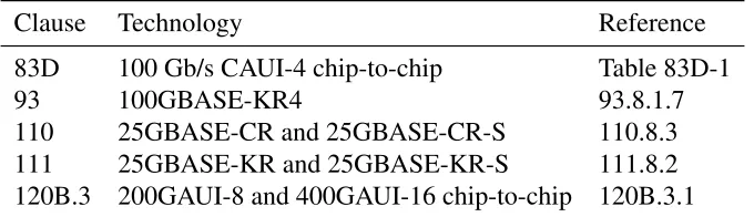
1.1 IEEE 802.3-2018 clauses that use Clause 92 TOJ tests. . . 2

3.1 List of hardware. . . 22

3.2 10 MHz PLL parameters reported on Keysight 86108B. . . 24

(13)

LIST OF FIGURES

Figure Page

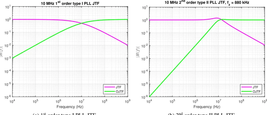
2.1 Example ideal PLL jitter transfer functions. . . 4

2.2 Example zero-crossing of a 100GBASE-KR4 calibrated stressed RX signal (pre-channel, no random interferer) generated by an Anritsu MP1900A and captured on a Keysight 86108B (CDR: 2nd_{order type II PLL,}_f 0 = 10 MHz, ftransition = 880 kHz). . . 6

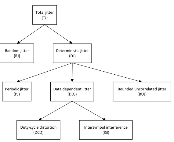
2.3 Jitter component hierarchy. . . 7

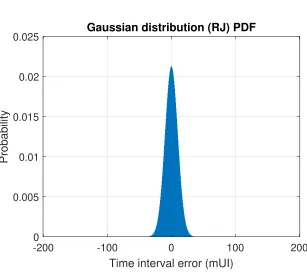
2.4 Example Gaussian PDF. . . 8

2.5 Example Gaussian CDF. . . 9

2.6 Example complementary error function. . . 10

2.7 Simulated Gaussian (RJ) PDF and bathtub curve (σ = 10mUI,µ= 0mUI). . . 13

2.8 Simulatedδ−δ(DJ) PDF and bathtub curve (σ = 1mUI,µ={−100,+50} mUI). . . 13

2.9 Simulatedδ−δ(DJ + RJ) PDF and bathtub curve (σ = 10mUI, µ={−100,+100}mUI). . . 14

2.10 Simulatedδ−δ(uniform DJ + RJ) PDF and bathtub curve (σ = 10mUI, µ={−100,+100}mUI). . . 15

2.11 Interpretation A ideal eye diagram. . . 18

2.12 Interpretation B ideal eye diagram. . . 19

2.13 Interpretation C ideal eye diagram. . . 20

3.1 TOJ test setup diagram. . . 23

(14)

3.3 TOJ convergence of a real device over number of zero-crossing histogram

samples (95% confidence over various sample ranges). . . 27

4.1 Comparison of EBUJ across combinations of jitter agressors and test definition interpretations. . . 30

4.2 Comparison of ERJ across combinations of jitter agressors and test definition interpretations. . . 31

4.3 Comparison of ETUJ across combinations of jitter agressors and test definition interpretations. . . 32

4.4 Falling edge zero-crossing histogram (SJ + BUJ comparison). . . 34

A.1 Zero-crossing histogram (SJ: off, BUJ: off, RJ: off). . . 39

A.2 Zero-crossing histogram (SJ: off, BUJ: off, RJ: on). . . 39

A.3 Zero-crossing histogram (SJ: off, BUJ: on, RJ: off). . . 40

A.4 Zero-crossing histogram (SJ: off, BUJ: on, RJ: on). . . 40

A.5 Zero-crossing histogram (SJ: on, BUJ: off, RJ: off). . . 40

A.6 Zero-crossing histogram (SJ: on, BUJ: off, RJ: on). . . 41

A.7 Zero-crossing histogram (SJ: on, BUJ: on, RJ: off). . . 41

A.8 Zero-crossing histogram (SJ: on, BUJ: on, RJ: on). . . 41

B.1 Bathtub curve (SJ: off, BUJ: off, RJ: off). . . 42

B.2 Bathtub curve (SJ: off, BUJ: off, RJ: on). . . 42

B.3 Bathtub curve (SJ: off, BUJ: on, RJ: off). . . 43

B.4 Bathtub curve (SJ: off, BUJ: on, RJ: on). . . 43

B.5 Bathtub curve (SJ: on, BUJ: off, RJ: off). . . 43

B.6 Bathtub curve (SJ: on, BUJ: off, RJ: on). . . 44

B.7 Bathtub curve (SJ: on, BUJ: on, RJ: off). . . 44

(15)

ABSTRACT

Efficient Characterization of Transmitter Output Jitter Components in

100GBASE-CR4 Ethernet

by

Paul Willis

University of New Hampshire, December, 2019

(16)

CHAPTER 1 INTRODUCTION

1.1 Rationale of testing telecommunications equipment

Implementers of high speed networks place value in reliability and interoperability among devices. It is useful to be able to plug two modules into each other and reliably have a low bit error rate (BER) link established. In order to guarantee this, there are performance metrics for transmitters and receivers that can be characterized and compared against some specification. It is the role of standards bodies to define the details of links and the performance metrics to be met. The Institute of Electrical and Electronics Engineers (IEEE) creates and maintains the Ethernet standard (IEEE 802.3). IEEE 802.3 is used in many high speed networks, as evidenced by vendors from various networking industries requesting the development of new clauses [1, p. 152].

Error correction coding (ECC) techniques are a common way to handle a certain amount of errors. If a link has a BER that is too high, then the effective throughput and latency of that link is impacted, even with the use of ECC. Receivers must be able to decode malformed signals and transmitters must be able to transmit clean signals. Jitter is an important component of transmitter characterization to meet BER goals. If the edges come too early or too late compared to the recovered clock’s sample time then the symbol could be sampled too close to the edge. If a symbol is sampled too far along an edge then the receiver will sample a symbol at the incorrect voltage and an error will occur.

1.2 Rationale of research

(17)

implement. However, the 100GBASE-CR4 transmitter output jitter (TOJ) measurement methodol-ogy is more involved compared to other test definitions in the 100GBASE-CR4 specification. The 100GBASE-CR4 TOJ tests use Gaussian fitting, which have specific assumptions of the measured data that must be recognized. While implementing 100GBASE-CR4 TOJ tests, it is possible to make decisions that result in inaccurate measurements or that result in the tests taking longer than necessary to perform. Additionally, while implementing 100GBASE-CR4 TOJ tests it is possible to misinterpret the test definition. The purpose of this thesis is to explore the choices that must be made by an implementer of the 100GBASE-CR4 TOJ tests and provides information on the behavior of the IEEE 802.3 clause 92 TOJ test definitions. The results of this thesis can be used to aid interpretation of device results and definitions of future jitter tests.

This thesis only examines the case of IEEE 802.3-2018 subclause 92.8.3.8.2Effective bounded

uncorrelated jitter and effective random jitter (EBUJ and ERJ). This test definition has been

adopted by other IEEE 802.3-2018 clauses listed in Table 1.1. This test definition is important because it is used by all 25 Gbps non-return to zero (NRZ) Ethernet technologies that operate over copper cable or backplane channels.

Table 1.1.IEEE 802.3-2018 clauses that use Clause 92 TOJ tests. Clause Technology Reference 83D 100 Gb/s CAUI-4 chip-to-chip Table 83D-1

93 100GBASE-KR4 93.8.1.7

(18)

CHAPTER 2 THEORY

2.1 Concepts of jitter

2.1.1 Definition of jitter

Jitter is the phase error of a signal compared against a reference clock with a spectrum greater than 10 Hz. Wander is defined as phase error of a signal compared against a reference clock with a spectrum less than 10 Hz [3, p. 1-3]. Most baseband communications systems embed clock information in the data signal. This removes the requirement of having an extra channel to distribute a clock signal at the expense of requiring line coding that guarantees a minimum number of transitions in any sequence of symbols, also known as transition density. Receivers reconstruct a clock signal from a received data signal using a clock and data recovery (CDR) circuit that is typically composed of a phase-locked loop (PLL) [4, p. 47]. PLLs can track phase error at frequencies less than than their loop filter bandwidth. Jitter at frequencies greater than the PLL loop filter bandwidth results in phase error between the reconstructed clock and the signal that the receiver samples.

A CDR’s jitter transfer function (JTF) is the ratio of the phase error at the CDR’s output to the phase error present in CDR’s input [5, p. 2]. The observed jitter transfer function (OJTF) is the inverse of the JTF. The JTF magnitude spectrum and OJTF magnitude spectrum of a given ideal system sum to unity (2.1) because a CDR should not apply gain to jitter. The OJTF magnitude spectrum is useful because it is the spectrum of jitter that is not tracked by a receiver’s CDR. Jitter in the OJTF passband negatively affects BER.

|OJ T F|= 1− |J T F| (2.1)

Figure 2.1 shows the JTF of two typical PLL implementations. 1st_{order PLLs have a less steep roll}

(19)

2nd order PLLs track high frequency jitter better than 1st order PLLs, but typically have an under-damped response. This underunder-damped response causes peaking in gain below the cutoff frequency, which causes jitter in the peaking band to affect the signal more. The choice between 1st and 2nd order PLLs is influenced by the expected jitter spectrum.

104 105 106 107 108 109

Frequency (Hz) 10-6

10-5 10-4 10-3 10-2 10-1 100

101 10 MHz 1

st

order type I PLL JTF

JTF OJTF

(a) 1st_{order type I PLL JTF.}

104 105 106 107 108 109

Frequency (Hz) 10-6

10-5 10-4 10-3 10-2 10-1 100 101

10 MHz 2nd order type II PLL JTF, f_z = 880 kHz

JTF OJTF

(b) 2nd_{order type II PLL JTF.}

Figure 2.1.Example ideal PLL jitter transfer functions.

The ability of CDRs to track low frequency phase error means wander is only an issue if the maximum frequency deviation of the received signal is outside of the CDR’s tracking range. The CDR tracking range is specified by two 100GBASE-CR4 tests:

• IEEE 802.3-2018 subclause 92.8.3.9Signaling rate rangefor transmitter • IEEE 802.3-2018 subclause 92.8.4.6Signaling rate rangefor receiver

(20)

is an example eye diagram captured with an equivalent time (ET) oscilloscope. It is possible to generate eye diagrams with data captures from real time (RT) oscilloscope, however it requires the collection of long sequences of data and a CDR implemented in post processing.

This thesis will refer to the edge crossings of two-level NRZ signals as zero-crossings. “Edge crossings” is a more general term that should be used with modulation schemes and/or technologies that have edge crossings that are not necessarily at zero volts.

The zero-crossing histogram is taken from−0.2unit interval (UI) to+0.2UI centered around the right edge mean zero-crossing time. UI is a time unit that is equivalent to the length of time of one symbol at a given symbol rate. This is the same time range that all other measurements in this document use. This zero-crossing histogram is the distribution of TIE values for the observed edges. 1 UI @ 25.78125 GBaud is 38.78 ps. In the case of Figure 2.2, t = 0 on the left edge of the plot. The left zero-crossing is at t = 0.3 UI (12.92 ps). The mean of the right zero-crossing is nominally at t = 1.3 UI (51.71 ps). The −0.2UI and +0.2 UI bounds used in the zero-crossing histogram are nominally at43.95 ps and59.47 ps, respectively. The actual bounds present in Figure 2.2 are slightly offset from these nominal values because the actual right edge zero-crossing mean is not at its nominal location of1.3UI from the left edge.

(21)

Eye diagram with 10 MHz Type II PLL

10 20 30 40 50 60

Time (ps) -600

-400 -200 0 200 400 600

Differential voltage (mV)

0 100 223 347 470 594 717 841 964 1087 1211

Samples per mV

ps

Zero-crossing

(a) Example eye diagram.

Zero-crossing histogram, bin size: 86.3 fs

40 45 50 55 60

Time (ps) 0

10 20 30 40 50 60 70 80

Number of samples per bin

(b) Example zero-crossing histogram. Figure 2.2. Example zero-crossing of a 100GBASE-KR4 calibrated stressed RX signal (pre-channel, no random interferer) generated by an Anritsu MP1900A and captured on a Keysight 86108B (CDR: 2nd_{order type II PLL,}_f

0 = 10 MHz,ftransition = 880 kHz).

2.1.2 Jitter decomposition

(22)

sources (aggressors) to a signal of interest (victim). BUJ is occasionally separated into periodic and non-periodic components, with non-periodic components being difficult to distinguish from RJ.

Total jitter (TJ)

Random jitter (RJ)

Deterministic jitter (DJ)

Periodic jitter (PJ)

Data dependent jitter (DDJ)

Bounded uncorrelated jitter (BUJ)

Duty‐cycle distortion (DCD)

Intersymbol interference (ISI)

Figure 2.3.Jitter component hierarchy.

2.2 Transmitter output jitter tests

(23)

ef-fective random jitter has fewer details than the original presentation, so the presentation is useful to reference when making implementation choices. IEEE-802.3 likely removed the details in the original presentation to not show a preference towards certain hardware solutions in test and mea-surement.

2.2.1 Gaussian distributions

The Gaussian distribution probability density function (PDF) is defined in (2.2). The Gaussian PDF is greater than zero for all real inputs: the tails are unbounded.

f x|µ, σ2= √ 1

2πσ2e

−(x−µ)2

2σ2 (2.2)

Gaussian distribution (RJ) PDF

-200 -100 0 100 200

Time interval error (mUI) 0

0.005 0.01 0.015 0.02 0.025

Probability

(24)

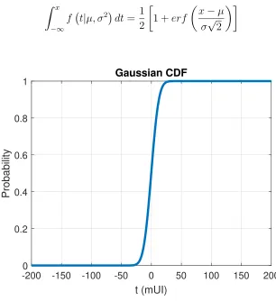
The Gaussian cumulative distribution function (CDF) is defined in (2.3).

Z x

−∞

f t|µ, σ2dt= 1

2

1 +erf

x−µ

σ√2

(2.3)

-200 -150 -100 -50 0 50 100 150 200

t (mUI) 0

0.2 0.4 0.6 0.8 1

Probability

Gaussian CDF

Figure 2.5. Example Gaussian CDF.

The Gaussian error function (erf) maps a range of a Gaussian distribution to the probability of that range. erf is defined in (2.4). erf, and by extension all functions based off of it, do not have closed form solutions.

erf(x) = √2

π Z x

0

(25)

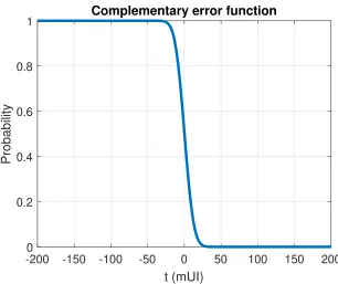
The complementary error function (erf c) is defined in (2.5). Due to Gaussian PDFs being symmetric about their mean, theerf cis equivalent to taking the CDF of a Gaussian distribution with the horizontal axis reversed (right to left instead of left to right).

erf c(x) = 1−erf(x) (2.5)

-200 -150 -100 -50 0 50 100 150 200

t (mUI) 0

0.2 0.4 0.6 0.8 1

Probability

Complementary error function

Figure 2.6. Example complementary error function.

The inverse complementary error function is defined in (2.6).

erf c(erf c−1(x)) = x (2.6)

erf c−1converts a Gaussian CDF to the range that it corresponds to. erf c−1 is used as a metric

of how Gaussian a distribution is. Using Equation (92-12) in IEEE 802.3-2018 (2.7), the BER scale of CDFs can be converted to Q.

(26)

Q(x) is directly proportional to erf c−1₍_x₎_{. If a random variable (RV) has a Gaussian}

com-ponent in its PDF, then the tail of that Gaussian comcom-ponent corresponds to high Q values. The higher the Q curve value, the further along the Gaussian tail the CDF is. The higher Q curve values correspond to confidence in lower BER values [6, p. 465]. These higher Q curve values are filled in by observing more samples.

2.2.2 Dual-Dirac model

The dual-Dirac (δ−δ) model is a method of splitting TJ into RJ and DJ [10, p. 3] [11, p. 1]. The δ−δ model assumes TJ is composed of two Gaussian distributions summed together. The

δ−δ model fits two Gaussian distributions from the tail regions on the left and right of the TIE histogram. The name “dual-Dirac” comes from the use of two Dirac delta functions convolved with Gaussian distributions. The time offset (mean of the Gaussian distributions) determines the magnitude of the measured DJ component. The standard deviation of the Gaussian distributions determines the magnitude of the measured RJ component. Theδ−δmodel allows extrapolation of RJ to predict TJ values at very low BER values while only needing to observe enough samples to fit the tails of the Gaussian distributions.

(27)

Theδ−δ model begins with an edge crossing PDF. Two CDFs are made from this PDF: one going from left to right and the other going from right to left (CDFL and CDFR).erf c−1_{is applied}

to the CDFs to generate Q curves:QLi andQRi.

If the region of the Q curve is high enough it should be outside of the bounds of DJ and be representative of histogram samples that are purely due to RJ. This purely RJ region can then be extrapolated to the low target BER without observing _BER3 samples. Observing _BER3 samples is necessary to be 95% confident that the actual BER is below the observed value [12, p. 15] when jitter is not decomposed into DJ and RJ. The ability to extrapolate RJ is the key benefit that the

δ−δmodel provides. The extrapolated Q curves are denoted asQlef tandQright. The maximum

Q value that DJ influences is dependent on the shape and amplitude of the DJ. The slope of the Q curve in the high Q region is determined by RJ. This is demonstrated in a simulated case where only RJ is present (Figure 2.7). In bathtub curves the right curve has 1 UI of time offset applied to it. The actual data used in calculations does not have this time offset applied to it and the mean of both left and right distributions is set to0 s.

Figure 2.7a is the PDF of a simulated edge crossing with Gaussian jitter applied to it. The horizontal axis is the time offset from the ideal crossing time in mUI: thousandths of a symbol time. The vertical axis is the probability of an edge arriving at a given time relative to a recovered clock.

Figure 2.7b is the bathtub curve of the simulated edge crossing histogram. QLiis the likelihood

of an edge on the left side of an eye diagram of occurring at a given time.QRiis the likelihood of

an edge on the right side of an eye diagram of occurring at a given time. The black dots indicate the points used to generate the linear fit curves:Qlef tandQright. This linear fit region is defined by

IEEE 802.3-2018 100GBASE-CR4 TOJ test definition. This region is assumed to be sufficiently outside of the bounds of DJ.

(28)

Gaussian distribution (RJ) PDF

-200 -100 0 100 200

Time interval error (mUI) 0 0.005 0.01 0.015 0.02 0.025 Probability

(a) Gaussian (RJ) PDF.

0 200 400 600 800 1000

time (mUI) 0 2 4 6 8 10 Q

Gaussian distribution (RJ) bathtub curve

QL_i

QR i QL

i/QRi linear fit region Q_left/Q_right

BER limit

(b) Gaussian (RJ) bathtub curve. Figure 2.7. Simulated Gaussian (RJ) PDF and bathtub curve (σ= 10mUI,µ= 0mUI).

The time offset (x-intercept) of a Q curve is equivalent to DJ. This is demonstrated in a sim-ulated case where only DJ is present (Figure 2.8). QLi is shifted by 100 mUI andQRi is shifted

by 50 mUI, corresponding to the eye closure caused by the DJ distribution centered around each Dirac delta function.

- distribution (DJ) PDF

-200 -150 -100 -50 0 50 100 150 200

Time interval error (mUI) 0 0.02 0.04 0.06 0.08 0.1 0.12 Probability

(a)δ−δ(DJ) PDF.

0 200 400 600 800 1000

time (mUI) 0 2 4 6 8 10 Q

- distribution (DJ) bathtub curve

QL i QR_i

QL_i/QR_i linear fit region

Q_left/Q_right

BER limit

(b)δ−δ(DJ) bathtub curve.

(29)

These two effects are independent of each other. This is demonstrated in a simulated case where both DJ and RJ is present (Figure 2.9). Both the slope and x-intercepts of the Q curves are influenced by the presence of RJ and DJ.

- distribution (DJ + RJ) PDF

-200 -100 0 100 200

Time interval error (mUI)

0 0.002 0.004 0.006 0.008 0.01 0.012

Probability

(a)δ−δ(DJ + RJ) PDF.

0 200 400 600 800 1000

time (mUI)

0

2

4

6

8

10

Q

- distribution (DJ + RJ) bathtub curve

QL_i

QR i QL

BER limit

(b)δ−δ(DJ + RJ) bathtub curve.

Figure 2.9. Simulatedδ−δ (DJ + RJ) PDF and bathtub curve (σ = 10mUI,µ={−100,+100}

mUI).

(30)

- distribution (uniform DJ + RJ) PDF

-200 -100 0 100 200

0.0005 0.001 0.0015 0.002 0.0025

Probability

(a)δ−δ(uniform DJ + RJ) PDF.

0 200 400 600 800 1000

time (mUI)

0

2

4

6

8

10

Q

- distribution (uniform DJ + RJ) bathtub curve

QL_i

QR i QL

BER limit

(b)δ−δ(uniform DJ + RJ) bathtub curve.

Figure 2.10. Simulated δ − δ (uniform DJ + RJ) PDF and bathtub curve (σ = 10 mUI, µ =

{−100,+100}mUI).

The time between the Q curves at a given BER is the expected horizontal eye opening at that BER. This type of plot is typically referred to as a bathtub curve. Bathtub curves have horizontal units in seconds or UI. Bathtub curves have vertical scales in logarithmic BER when displaying CDFs. Bathtub curves have inverted vertical scales when displaying Q curves to mimic the appear-ance of a BER scale bathtub [10, p. 10].

Estimated bounded uncorrelated jitter (EBUJ) is defined in Equation (92-18) in IEEE 802.3-2018 (2.8). It is assumed that the Q curves will have the same characteristics as typical bathtub curves. That is to say: Qlef t is a negatively sloped (mlef t < 0) line with a positive x-intercept

(blef t >0) andQright is a positively sloped (mright > 0) line with a negative x-intercept (bright <

0).

EBU J = blef t

mlef t

− bright

mright

(31)

ERJ = mlef t−mright

2×mlef t×mright

(2.9)

Estimated total uncorrelated jitter (ETUJ) is defined in Equation (92-19) in IEEE 802.3-2018 (2.10). The reason ERJ is multiplied by 7.9 is to extrapolate from the RMS RJ value to BER= 10−15(2.11).

ET U J = 7.9×ERJ ×EBU J (2.10)

Q 10−15≈7.9 (2.11) The 100GBASE-CR4 TOJ tests only define measurement limits for EBUJ and ETUJ. This thesis reports EBUJ, ETUJ, and ERJ. EBUJ and ETUJ are reported to evaluate measured results against the test limit. ERJ is reported to evaluate how well theδ−δmodel is working.

2.2.3 Test methodology

IEEE 802.3-2018 subclause 92.8.3.8.2 defines the math operations necessary to go from zero-crossing histograms to EBUJ, ERJ, and estimated total uncorrelated jitter (ETUJ). It is important to note that ETUJ is not the same as TJ. TJ includes jitter components that are correlated with the data signal: DDJ. TJ at a given BER is also directly observed with 95% confidence by observing

3

BER samples whereas ETUJ is an extrapolation based on theδ−δ model. The IEEE 802.3-2018

subclause 92.8.3.8.2 test definition removes DDJ by only measuring jitter on specific edges and subtracting the mean time offset. Any DDJ should appear as a static time offset in the TIE for any one specific edge in a repeating data pattern. The mean jitter of the edges of interest are set to zero so, that any jitter component that tracks the data pattern is removed. This assumption is accurate because the test methodology involves only taking zero-crossing histograms on specific edges in a PRBS9 (Pseudo random binary sequence,29−1bits long) test pattern:

(32)

These selected edges are considered “lone edges” because there are no other transitions within a few symbols. In the PRBS9 test pattern these two subsequences have the longest runs of symbols preceding and following the transition of interest. EBUJ is an estimate of PJ and BUJ. ERJ is calcu-lated by taking the linear regression of the Q curves at CDF ranges 2.5·10−2_{to 10}−3_{, establishing}

the expected bound of DJ in each of the two Gaussian distributions in theδ−δ model. ETUJ is the combination of EBUJ and ERJ extrapolated to a BER of 10−15_{. Using Equation (92-12) in}

IEEE 802.3-2018, the BER scale of CDFs can be converted to Q (2.7). The Q scale CDF range of interest is1.96< Q <3.09. The Q scale of the target BER is7.94.

2.3 Interpretation of test definition

The first sentence in IEEE 802.3-2018 subclause 92.8.3.8.2 Effective bounded uncorrelated

jitter and effective random jitterstates:

“Effective bounded uncorrelated jitter and effective random jitter are measured on each of two specific transitions in a PRBS9 pattern (see 83.5.10).”

(33)

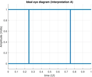
Interpretation A The zero-crossing histograms should be sample-wise summed together into a single PDF. The timebases of the two histograms should be combined by lin-early interpolating the PDFs to a common set of bins. QLi and QRi is

gen-erated using the singular resultant histogram. This interpretation is explicitly described in a later TOJ definition: IEEE 802.3-2018 subclause 120D.3.1.8.1

J4u andJRM S jitter. This test definition goes into greater detail about how to

do this combination for PAM4 signaling.Interpretation Ais the equivalent of averaging the left and right zero-crossings of an eye diagram made from lone edges and duplicating the resultant zero-crossing on the left and the right of the eye diagram.

0 0.1 0.2 0.3 0.4 0.5 0.6 0.7 0.8 0.9 1

time (UI) 0

0.2 0.4 0.6 0.8 1

Amplitude (Volts)

Ideal eye diagram (interpretation A)

(34)

Interpretation B The zero-crossing histograms should be kept separate. QLi is generated using

one histogram andQRi is generated by using the other histogram. There are

two configurations for this interpretation:

1. The rising edge histogram is used to generateQLi and the falling edge

histogram is used to generateQRi.

2. The falling edge histogram is used to generate QLi and the rising edge

histogram is used to generateQRi.

Both configurations are analyzed and the worst case values are chosen. Inter-pretation B is the equivalent of making an eye diagram with the left zero-crossing as a lone rising/falling edge and the right zero-zero-crossing as a lone falling/rising edge.

0 0.1 0.2 0.3 0.4 0.5 0.6 0.7 0.8 0.9 1

time (UI)

0 0.5 1

Amplitude (Volts)

Ideal eye diagram (interpretation B, positive pulse)

0 0.1 0.2 0.3 0.4 0.5 0.6 0.7 0.8 0.9 1

time (UI)

0 0.5 1

Amplitude (Volts)

Ideal eye diagram (interpretation B, negative pulse)

(35)

Interpretation C The zero-crossing histograms should be kept separate and the TOJ values should be calculated for each histogram. The worst case values for each mea-surement are the recorded results. Interpretation Cis the equivalent of taking one lone edge and constructing an eye diagram by duplicating the edge on the left and the right.

0 0.1 0.2 0.3 0.4 0.5 0.6 0.7 0.8 0.9 1

time (UI)

0 0.5 1

Amplitude (Volts)

Ideal eye diagram (interpretation C, rising edge)

0 0.1 0.2 0.3 0.4 0.5 0.6 0.7 0.8 0.9 1

time (UI)

0 0.5 1

Amplitude (Volts)

Ideal eye diagram (interpretation C, falling edge)

Figure 2.13.Interpretation C ideal eye diagram.

2.3.1 Comparison of interpretations

(36)

CHAPTER 3 SETUP

3.1 Oscilloscope choice

It is possible to implement 100GBASE-CR4 TOJ tests on RT oscilloscopes. A CDR can be implemented in post processing to produce the clock signal necessary to generate zero-crossing histograms. There are two edges of interest in every PRBS9 pattern (511 bits). 766,500 symbols would have to be captured in order to collect 3,000 histogram samples. At 4 samples per UI, 8 bits per voltage sample, and 1 double floating point precision time sample this would result in a

27.6 MBuncompressed file. This is a reasonable file size, but the CDR code would have to be well optimized to keep the post processing computation time to a reasonable length.

ET oscilloscopes can trigger on a repeating pattern. The time range can be made very small so that the only sampled data is near the zero-crossings of interest. ET oscilloscopes are limited in how many samples per second they can store so reducing the horizontal range provides the benefit of reducing test time. The voltage scale can also be reduced to increase voltage precision. This was not done during this testing to avoid potential artifacts due to voltage rail clipping. Using an ET oscilloscope with a zoomed in time range allows for the collection of a high precision TIE histogram quickly made on the oscilloscope that is only a fewkBin size and does not require post processing to reconstruct a reference clock. This reduces post processing computation and file size requirements, increases time domain precision, and potentially decreases overall test time. This technique comes at the cost of flexibility in implementing different CDRs in post processing. The exact time information of each sample is not kept, but only the zero-crossing histogram relative to the hardware CDR output is retained.

(37)

The speed of the test is limited by the trigger rate of oscilloscopes (typically less than a thousand a second). In order to directly observe a BER of 10−15 with a confidence of 95%, 3×1015 jitter samples need to be collected [12, p. 15]. With an oscilloscope with a sample fill rate of 1,000 samples/s, the tester would need to collect samples for 95,129 years. Theδ−δmodel allows the jitter to be characterized with many fewer samples. The exact number of samples depends on the region of Q used to characterize RJ. In the case of 100GBASE-CR4 tests only a few thousand samples are needed, so the test time is reduced to less than a minute.

IEEE 802.3-2018 subclause 92.8.3.8 states:

“The effect of a single-pole high-pass filter with a3 dBfrequency of10 MHzis applied to the jitter.”

This is interpreted as a specification for the CDR used to measure jitter. The effect of a high-pass filter is applied to the jitter by the ET oscilloscope’s CDR OJTF.

3.2 Hardware used

Table 3.1.List of hardware.

Equipment Manufacturer Model Software

version

Serial number

Oscilloscope Keysight 86108B N/A MY52130389

Oscilloscope

mainframe Keysight

DCA-X

86100D A.06.01.68 MY57350354 Phase

shifters

Spectrum

Elektrotechnik LS-P150-HFHM N/A

CH1: 5306 CH2: 5307

DC blocks Picosecond

Pulse Labs 5501A N/A

CH1: 8567 CH2: 8565 2.4mm to

SMA adapter Keysight 11901C N/A

CH1: 20724 CH2: 35601

SMA cables Huber+Suhner Sucoflex

104PE N/A

CH1: 255105016 CH2: 255105019

(38)

BERT

Output

Oscilloscope

Phase shifters SMA adapters DC blocks Input

Figure 3.1. TOJ test setup diagram.

3.2.1 Explanation

A Keysight ET oscilloscope was used because it is the highest performance ET oscilloscope available to the University of New Hampshire InterOperability Laboratory (UNH-IOL) during this research. It is expected that comparable oscilloscopes from other manufacturers would yield com-parable results to those in this thesis. The use of phase shifters is recommended by Keysight when measuring signals with symbol rates (SR) above 10 Gbps on the 86108B. The phase-matched SMA cables have approximately5 ps of skew, which can be corrected to less than 200 fsof skew with phase shifters. The rated jitter noise floor of the 86108B is < 70 fs. DC blocks are used dur-ing 100GBASE-CR4 testdur-ing because the maximum allowed DC offset is above the oscilloscope’s power rating. The DC blocks and SMA cables are rated for 26.5 GHzand limit the performance of the system. SMA’s bandwidth limitation of26.5 GHzis acceptable for this testing but2.4 mm

(39)

According to the 86108B programmer’s guide [13, p. 158] the order and type of the ET oscil-loscope’s built-in CDR is an underdamped 2nd order type 2 PLL and is not adjustable. This is not compliant with the 100GBASE-CR4 specification and does decrease the amount of low frequency jitter present in the measurement. The ET oscilloscope’s built-in CDR has four available transition frequency settings atf0 = 10 MHzshown in Table 3.2. The 86108B programmer’s guide states:

“The Type-2 transition frequency indicates the frequency below which the second in-tegrator in the loop starts to provide extra gain.”

The transition frequency was chosen to be880 kHzas a balance between OJTF peaking and rolloff. Note that the list of available transition frequency values present on the 86108B used are not the same as those listed in the 86108B programmer’s guide. It is possible that other instances of this oscilloscope could have different transition frequency options than those listed in Table 3.2.

Table 3.2.10 MHz PLL parameters reported on Keysight 86108B.

ftransition (kHz) Peaking (dB)

12 0

320 0.5

880 1.1

2800 2.1

Both ET and RT oscilloscopes may commonly have a jitter characterization mode that directly measures zero-crossing histograms with high sample rates. These modes often do not have a way to specify a specific edge in a pattern to measure.

3.3 Calibration values

(40)

performed. SJ was calibrated at150 MHz. BUJ was calibrated with a PRBS7 pattern transmitting at 12.5 Gbps. Table 3.3 is a list of the measured calibrated jitter values. Figure 3.2 is the eye diagram of the calibrated signal with all three jitter aggressors applied.

Table 3.3.Calibrated jitter component values. jitter

component

calibrated value (mUI) RJ (RMS) 10

BUJ 35

SJ 100

These values are slightly above the limit for TOJ tests. With all three aggressors applied the applied BUJ is 135 mUI and applied TJ@BER= 10−15is 214 mUI. The EBUJ maximum limit is 100 mUI. The ETUJ maximum limit is 180 mUI.

Calibrated 100GBASE-CR4 pre-channel eye diagram

10 20 30 40 50 60 70

Time (ps)

-1000 -800 -600 -400 -200 0 200 400 600 800 1000

Differential voltage (mV)

0 10 56 103 149 195 242 288 334 381 427

Samples per mV

ps

Figure 3.2. Eye diagram of a 100GBASE-CR4 calibrated stressed RX signal (pre-channel) gen-erated by an Anritsu MP1900A and captured on a Keysight 86108B (CDR: 2nd_{order type II PLL,}

(41)

3.4 Histogram optimization

3.4.1 Number of samples

The original TOJ presentation [9, p. 10] says each zero-crossing histogram has at least 20,000 samples. A data set from a real DUT was collected during early research. This data set was used to perform a TOJ convergence analysis (Figure 3.3). The methodology of collecting histograms on ET oscilloscopes had not been discovered yet, so this data was built up from capturing many instances of the entire test pattern. A MATLAB based post processing CDR based on applying a linear regression to the count of edges over edge times was used.

The linear fit CDR works by drawing an ideal Baud line with a horizontal axis of time and a vertical axis of number of UI. Each edge time is assigned a UI value that places it closest to the ideal Baud line. A linear regression is calculated on the edge time points. The slope of this linear regression is the actual average SR. The linear regression CDR does not track low frequency jitter. The data is broken into blocks to remove low frequency jitter components. The block size was chosen to be _{10 MHz}1 to not have frequencies below10 MHzin the OJTF. The methodology of capturing instances of the entire test pattern and applying a post processing CDR is less accurate than the direct histogram methodology but the conclusion from the convergence test applies to the direct histogram methodology.

(42)

real data even though negative jitter values cannot exist in the real world. This indicates that the mean of one of the Gaussian distributions in theδ−δmodel is negative when it is expected to be positive or vice-versa.

0 2000 4000 6000 8000 10000 Number of samples

0 5 10 15 20 25 30 mUI EBUJ convergence EBUJ EBUJ PDF

3.0k-10k samples, 95% confidence 5.0k-10k samples, 95% confidence 7.5k-10k samples, 95% confidence

(a) EBUJ convergence.

0 5 10 15 20 25 30 mUI ERJ convergence ERJ ERJ PDF

(b) ERJ convergence.

100 110 120 130 140 150 160 mUI ETUJ convergence ETUJ ETUJ PDF

(c) ETUJ convergence. Figure 3.3. TOJ convergence of a real device over number of zero-crossing histogram samples (95% confidence over various sample ranges).

3.4.2 Bin size

The original TOJ presentation [9, p. 10] says that the histogram resolution shall be no coarser than 50 fs/bin but no finer than 5 fs/bin. A histogram width of 400 mUI was chosen to be able to observe histogram samples from signals with RJ values more than twice the specification limit. The horizontal resolution of the oscilloscope was set to its maximum: 65,536 points per waveform. However, histograms that the oscilloscope returns have a fixed number of bins: 751. This results in20.7 fs/bin, which is in the middle of the range recommended in the original TOJ presentation.

3.5 Measurements taken

(43)

1. CDR lock and pattern lock were acquired on the ET oscilloscope.

2. Apply a fourth-order Bessel-Thomson low-pass filter to the signal as per IEEE 802.3-2018 92.8.3 using the oscilloscope built-in math functions.

3. The voltage range was set to200 mV/division to avoid clipping.

4. The edge of interest was located in the data pattern and placed in the display range.

5. A zero-crossing histogram was taken to determine the mean of the edge of interest relative to the pattern trigger.

6. The time scale was set to±200mUI about the mean crossing time with 65,536 samples per waveform.

(44)

CHAPTER 4 RESULTS

4.1 Data

(45)

SJ

off

BUJ off RJ

off

SJ

off

BUJ off RJ

on SJ off BU J on RJ of f SJ off BUJ on RJ on SJ on

BUJ off RJ

off

SJ

on

BUJ off RJ

on SJ on BUJ on RJ off SJ on BU J on RJ on A 1.2 3.7 54.6 46.9 51. 5 37.7 34.2 31.5 B 0.4 5.2 63.3 42.5 52. 1 43.4 33.7 39.7 C 0.8 6.0 63.4 45.6 52 .2 37.3 44.4 36.6 0.0 10.0 20.0 30.0 40.0 50.0 60.0 70.0 mUI

E

B

U

J

C

o

m

p

a

ri

so

n

(46)

SJ off BUJ off RJ off SJ off BUJ off RJ on SJ of f BUJ on RJ off SJ off BUJ on RJ on SJ on BUJ off RJ off SJ on BUJ off RJ on SJ on BUJ on RJ off SJ on BUJ on RJ on A 3.1 7.5 14.9 18.7 4.6 10.7 26.1 27.0 B 3.5 8.5 13.9 20.2 4.7 12.7 27.7 29.7 C 3.7 8.7 14.9 21.3 4.8 11.5 30.9 28.6 0. 0 5.0 10.0 15.0 20.0 25.0 30.0 35.0 mUI

E

R

J

C

o

m

p

a

ri

so

n

(47)

SJ off BUJ off RJ off SJ off BUJ off RJ on SJ off BUJ on RJ off SJ off BUJ on RJ on SJ on BUJ off RJ off SJ on BUJ of f RJ on SJ on BUJ on RJ off SJ on BUJ on RJ on A 25.8 63.3 172.6 194.8 87.6 122.6 240.7 245.0 B 26.8 66.7 169.3 201.5 87.9 128.4 245.5 255.9 C 28.2 67.4 177. 6 202. 9 88.9 124. 5 259. 7 250. 5 0.0 50. 0 100.0 150 .0 200 .0 250 .0 300 .0 mUI

E

T

U

J

C

o

m

p

a

ri

so

n

(48)

4.2 Discussion

All three interpretations correlate with each other across all jitter aggressor configurations. For a given configuration of jitter aggressors all three interpretations are within 10 mUI of each other, with the largest deviations being in EBUJ. Note that SJ is a component of BUJ. EBUJ increased when SJ was applied. Theδ−δmodel does not perfectly separate RJ from DJ. When SJ and BUJ were enabled, the ERJ was measured to be10−20mUI higher than with all aggressors disabled. This observation corroborates simulation [14, p. 8].

In cases where large amounts of DJ are present (Figure A.7, Figure B.7, Figure A.8, Figure B.8)

Qlef tandQrightare not symmetric. Qlef tandQrightshould be symmetric if the Q linear fit region

(49)

Falling edge histogram (3072 samples, bin size: 21.7 fs) SJ:off BUJ:on RJ:off, interpretation B

-200 -150 -100 -50 0 50 100 150 200 Time interval error (mUI)

0 10 20 30 40

(a) SJ: off, BUJ: on, RJ: off.

Falling edge histogram (3063 samples, bin size: 21.7 fs) SJ:on BUJ:off RJ:off, interpretation B

0 10 20 30 40 50

(b) SJ: on, BUJ: off, RJ: off.

Falling edge histogram (3062 samples, bin size: 21.7 fs) SJ:on BUJ:on RJ:off, interpretation B

0 5 10 15 20 25 30

(c) SJ: on, BUJ: on, RJ: off. Figure 4.4.Falling edge zero-crossing histogram (SJ + BUJ comparison).

Figure 4.1 shows that adding both BUJ and SJ to the jitter distribution resulted in a lower EBUJ than when only SJ is present. Figure 4.4 shows a comparison of falling edge zero-crossing histograms with BUJ on and SJ off, BUJ off and SJ on, and BUJ on and SJ on. This comparison highlights the difference in jitter distribution shape between these three cases. The jitter distribution shape is more Gaussian when both deterministic jitter sources were present than when only one was present. The Dirac Delta functions of theδ−δmodel are closer to the center and the standard deviation of the Gaussian functions is larger. This effect is an example of the central limit theorem, however the deterministic components are still bounded in nature. If the Q curve was extrapolated from regions of the edge-crossing histogram that were outside of the deterministic jitter’s bound, then this effect would not affect the estimated jitter values.

(50)

CHAPTER 5 CONCLUSION

5.1 Evaluation

This ET oscilloscope-based implementation satisfies IEEE 802.3-2018 subclause 92.8.3.8.2, with the exception of the JTF rolloff being 2nd order instead of 1st order. The TOJ test definition can cause pessimistic estimations of ERJ and EBUJ, and optimistic estimations of EBUJ. The magnitude of the error is dependent on the shape of the DJ distribution. The chance of this error could be reduced by changing the test definition to apply the linear fit in a different way. The range of Q values could be statically set to be higher, though this requires an exponential increase in the number of samples required to be observed to define the higher values of Q (Equation 2.7)

The estimate of 3,000 samples per histogram was made in the interest of reducing test time but pushes the limit of what is acceptable forInterpretation BandInterpretation C. 5,000 to 10,000 histogram samples would provide more confidence in scenarios where BUJ is large. It is possible that a device with large amounts of non-periodic BUJ that marginally fails ETUJ would pass an ETUJ test that used higher values of Q to characterize RJ. A failing TOJ result of a device could be a false positive indicator for interoperability issues.

(51)

5.2 Future work

5.2.1 Post processing CDR

More advanced and efficient post processing CDR code would increase the JTF performance in RT oscilloscope-based implementations relative to windowed linear fit CDR. A high Q bandpass filter CDR [4, p. 54] is simple to implement in software. A high Q bandpass filter CDR is a bandpass filter of the received data signal with a center frequency of the SR fundamental frequency and a bandwidth of the loop filter bandwidth. For 100GBASE-CR4 this would be a bandpass filter withQ = 1,289. Issues related to high Q filtering in software are: the precision limit of double-precision floating-point, and the need to align the clock phase to the data. The clock offset could be calculated by generating an eye diagram and taking the mean of the zero crossing histogram across one UI (two edges).

More advanced linear fit CDR windowing techniques are also possible. A sliding window linear fit CDR that combines multiple results for a single clock time using a weighting function could be implemented to have tighter control over the JTF. The average symbol rate has the most error at the edges of the window, so those regions would be given the lowest weight. The width of the window would likely dictate the cutoff frequency of the JTF. The window function shape would likely influence the passband and stopband characteristics. This sliding window linear fit CDR should be explored mathematically and verified empirically to demonstrate if it is possible to generate a CDR with an arbitrary cutoff frequency and passband shape.

(52)

LIST OF REFERENCES

[1] R. Rabinovich, “40gb/s 100gb/s ethernet long-reach host board channel design,”IEEE

Com-munications Magazine, vol. 51, no. 11, pp. 152–158, Nov 2013.

[2] “IEEE standard for ethernet,”IEEE Std 802.3-2018 (Revision of IEEE Std 802.3-2015), pp. 1–5600, Aug 2018. [Online]. Available: https://doi.org/10.1109/IEEESTD.2018.8457469 [3] R. Neil, “Understanding jitter and wander measurements and standards,” Agilent

Technologies, Tech. Rep. 5988-6254EN, Feb 2003. [Online]. Available: http://literature.cdn. keysight.com/litweb/pdf/5988-6254EN.pdf

[4] M. Hsieh and G. E. Sobelman, “Architectures for multi-gigabit wire-linked clock and data recovery,”IEEE Circuits and Systems Magazine, vol. 8, no. 4, pp. 45–57, Apr 2008.

[5] M. Schnecker, “Jitter transfer measurement in clock circuits,” LeCroy Corporation, Tech. Rep., Feb 2009. [Online]. Available: http://cdn.teledynelecroy.com/files/whitepapers/ designcon2009_lecroy_jitter_transfer_measurement_in_clock_circuits.pdf

[6] J. Moreira and H. Werkmann, An Engineer’s Guide to Automated Testing of High-Speed

Interfaces, 1st ed. Artech House, 2010.

[7] A. Kuo, R. Rosales, T. Farahmand, S. Tabatabaei, and A. Ivanov, “Crosstalk bounded uncorrelated jitter (BUJ) for high-speed interconnects,” IEEE Transactions on

Instrumentation and Measurement, vol. 54, no. 5, pp. 1800–1810, Oct 2005. [Online].

Available: https://doi.org/10.1109/tim.2005.855101

[8] P. Zivny, “Jitter and noise measurements in presence of crosstalk and 802.3bj,” in100 Gb/s

Backplane and Copper Cable Task Force 2011 Chicago Meeting Materials. IEEE, Sep

2011. [Online]. Available: http://www.ieee802.org/3/bj/public/sep11/zivny_01_0911.pdf [9] P. Zivny and C. Moore, “802.3bj d2.1 transmitter output jitter specification for nrz pmds,” in

100 Gb/s Backplane and Copper Cable Task Force 2013 Geneva Meeting Materials. IEEE,

Jul 2013. [Online]. Available: http://ieee802.org/3/bj/public/jul13/zivny_3bj_01a_0713.pdf [10] R. Stephens, “White paper: Jitter analysis: The dualdirac model, rj/dj, and

q-scale,” Agilent Technologies, Tech. Rep., Dec 2004. [Online]. Available: https: //www.keysight.com/upload/cmc_upload/All/dualdirac1.pdf

[11] ——, “White paper: What the dual-dirac model is and what it is not,” Tektronix, Tech. Rep. 55W-21988-0, Oct 2006. [Online]. Available: https://ransomsnotes.com/index_htm_ files/RansomStephensJitter360Pt2DualDirac.pdf

(53)

[13] Keysight 86100A/B/C/D Wide-Bandwidth Oscilloscope Programmer’s Guide, 11th ed., Keysight Technologies, Apr 2015. [Online]. Available: https://www.keysight.com/upload/ cmc_upload/All/86100_Programming_Guide.pdf

[14] C. Moore, “Experiments with simulated jitter,” in 100 Gb/s Backplane and Copper Cable

Task Force 2014 Indian Wells Meeting Materials. IEEE, Jan 2014. [Online]. Available:

(54)

APPENDIX A

ZERO-CROSSING HISTOGRAM FIGURES

Combined edge histogram (6100 samples, bin size: 25.9 fs) SJ:off BUJ:off RJ:off, interpretation A

0 100 200 300 400 500

(a) Combined edge histogram.

Falling edge histogram (3059 samples, bin size: 21.7 fs) SJ:off BUJ:off RJ:off, interpretation B

-200 -150 -100 -50 0 50 100 150 200

Time interval error (mUI) 0 50 100 150 200 250

(b) Falling edge histogram.

Rising edge histogram (3041 samples, bin size: 21.7 fs) SJ:off BUJ:off RJ:off, interpretation B

-200 -150 -100 -50 0 50 100 150 200

(c) Rising edge histogram. Figure A.1. Zero-crossing histogram (SJ: off, BUJ: off, RJ: off).

Combined edge histogram (6124 samples, bin size: 25.9 fs) SJ:off BUJ:off RJ:on, interpretation A

-200 -150 -100 -50 0 50 100 150 200

50 100 150 200

Falling edge histogram (3085 samples, bin size: 21.7 fs) SJ:off BUJ:off RJ:on, interpretation B

-200 -150 -100 -50 0 50 100 150 200

Rising edge histogram (3039 samples, bin size: 21.7 fs) SJ:off BUJ:off RJ:on, interpretation B

-200 -150 -100 -50 0 50 100 150 200

(55)

Combined edge histogram (6107 samples, bin size: 25.9 fs) SJ:off BUJ:on RJ:off, interpretation A

-200 -150 -100 -50 0 50 100 150 200

Time interval error (mUI) 0 10 20 30 40 50 60 70

Falling edge histogram (3072 samples, bin size: 21.7 fs) SJ:off BUJ:on RJ:off, interpretation B

0 10 20 30 40

Rising edge histogram (3035 samples, bin size: 21.7 fs) SJ:off BUJ:on RJ:off, interpretation B

0 5 10 15 20 25 30 35

(c) Rising edge histogram. Figure A.3.Zero-crossing histogram (SJ: off, BUJ: on, RJ: off).

Combined edge histogram (6097 samples, bin size: 25.9 fs) SJ:off BUJ:on RJ:on, interpretation A

0 10 20 30 40 50 60

Falling edge histogram (3036 samples, bin size: 21.7 fs) SJ:off BUJ:on RJ:on, interpretation B

0 5 10 15 20 25 30 35

Rising edge histogram (3061 samples, bin size: 21.7 fs) SJ:off BUJ:on RJ:on, interpretation B

0 5 10 15 20 25 30 35

(c) Rising edge histogram. Figure A.4.Zero-crossing histogram (SJ: off, BUJ: on, RJ: on).

Combined edge histogram (6122 samples, bin size: 25.9 fs) SJ:on BUJ:off RJ:off, interpretation A

-200 -150 -100 -50 0 50 100 150 200

Falling edge histogram (3063 samples, bin size: 21.7 fs) SJ:on BUJ:off RJ:off, interpretation B

0 10 20 30 40 50

Rising edge histogram (3059 samples, bin size: 21.7 fs) SJ:on BUJ:off RJ:off, interpretation B

0 10 20 30 40 50

(56)

Combined edge histogram (6133 samples, bin size: 25.9 fs) SJ:on BUJ:off RJ:on, interpretation A

-200 -150 -100 -50 0 50 100 150 200

Time interval error (mUI) 0 10 20 30 40 50 60 70

Falling edge histogram (3051 samples, bin size: 21.7 fs) SJ:on BUJ:off RJ:on, interpretation B

0 10 20 30 40

Rising edge histogram (3082 samples, bin size: 21.7 fs) SJ:on BUJ:off RJ:on, interpretation B

0 10 20 30 40

(c) Rising edge histogram. Figure A.6.Zero-crossing histogram (SJ: on, BUJ: off, RJ: on).

Combined edge histogram (6120 samples, bin size: 25.9 fs) SJ:on BUJ:on RJ:off, interpretation A

0 10 20 30 40 50 60

Falling edge histogram (3062 samples, bin size: 21.7 fs) SJ:on BUJ:on RJ:off, interpretation B

0 5 10 15 20 25 30

Rising edge histogram (3058 samples, bin size: 21.7 fs) SJ:on BUJ:on RJ:off, interpretation B

0 5 10 15 20 25 30 35

(c) Rising edge histogram. Figure A.7.Zero-crossing histogram (SJ: on, BUJ: on, RJ: off).

Combined edge histogram (6121 samples, bin size: 25.9 fs) SJ:on BUJ:on RJ:on, interpretation A

0 10 20 30 40 50

Falling edge histogram (3045 samples, bin size: 21.7 fs) SJ:on BUJ:on RJ:on, interpretation B

0 5 10 15 20 25 30

Rising edge histogram (3076 samples, bin size: 21.7 fs) SJ:on BUJ:on RJ:on, interpretation B

0 5 10 15 20 25 30

(57)

APPENDIX B

BATHTUB CURVE FIGURES

0 200 400 600 800 1000

time (mUI) 0 2 4 6 8 10 Q

Combined edge bathtub curve (6100 samples, bin size: 25.9 fs) SJ:off BUJ:off RJ:off, interpretation A

QL_i

QR_i

Q

left/Qright

BER limit

(a) Combined edge bathtub curve.

0 200 400 600 800 1000

time (mUI) 0 2 4 6 8 10 Q

Fall(L) / Rise(R) bathtub curve (3059 / 3041 samples, bin size: 21.7 / 21.7 fs)

SJ:off BUJ:off RJ:off, interpretation B

QL_i

QR_i

Q

left/Qright

BER limit

(b) Fall(L) Rise(R) bathtub curve.

0 200 400 600 800 1000

time (mUI) 0 2 4 6 8 10 Q

Rise(L) / Fall(R) bathtub curve (3041 / 3059 samples, bin size: 21.7 / 21.7 fs)

SJ:off BUJ:off RJ:off, interpretation B

QL_i

QR_i

Q

left/Qright

BER limit

(c) Rise(L) Fall(R) bathtub curve. Figure B.1. Bathtub curve (SJ: off, BUJ: off, RJ: off).

0 200 400 600 800 1000

time (mUI) 0 2 4 6 8 10 Q

Combined edge bathtub curve (6124 samples, bin size: 25.9 fs) SJ:off BUJ:off RJ:on, interpretation A

QL_i

QR i QL

i/QRi linear fit region

Q_left/Q_right

BER limit

0 200 400 600 800 1000

time (mUI) 0 2 4 6 8 10 Q

SJ:off BUJ:off RJ:on, interpretation B

QL_i

QR i QL

Q_left/Q_right

BER limit

0 200 400 600 800 1000

time (mUI) 0 2 4 6 8 10 Q

SJ:off BUJ:off RJ:on, interpretation B

QL_i

QR i QL

Q_left/Q_right

BER limit

(58)

0 200 400 600 800 1000 time (mUI) 0 2 4 6 8 10 Q

Combined edge bathtub curve (6107 samples, bin size: 25.9 fs) SJ:off BUJ:on RJ:off, interpretation A

QL_i

QR i QL

Q_left/Q_right

BER limit

0 200 400 600 800 1000

time (mUI) 0 2 4 6 8 10 Q

SJ:off BUJ:on RJ:off, interpretation B

QL_i

QR i QL

Q_left/Q_right

BER limit

0 200 400 600 800 1000

time (mUI) 0 2 4 6 8 10 Q

SJ:off BUJ:on RJ:off, interpretation B

QL_i

QR i QL

Q_left/Q_right

BER limit

(c) Rise(L) Fall(R) bathtub curve. Figure B.3.Bathtub curve (SJ: off, BUJ: on, RJ: off).

0 200 400 600 800 1000

time (mUI) 0 2 4 6 8 10 Q

Combined edge bathtub curve (6097 samples, bin size: 25.9 fs) SJ:off BUJ:on RJ:on, interpretation A

QL i

QR_i

Q

left/Qright

BER limit

0 200 400 600 800 1000

time (mUI) 0 2 4 6 8 10 Q

SJ:off BUJ:on RJ:on, interpretation B

QL i

QR_i

Q

left/Qright

BER limit

0 200 400 600 800 1000

time (mUI) 0 2 4 6 8 10 Q

SJ:off BUJ:on RJ:on, interpretation B

QL i

QR_i

Q

left/Qright

BER limit

(c) Rise(L) Fall(R) bathtub curve. Figure B.4.Bathtub curve (SJ: off, BUJ: on, RJ: on).

0 200 400 600 800 1000

time (mUI) 0 2 4 6 8 10 Q

Combined edge bathtub curve (6122 samples, bin size: 25.9 fs) SJ:on BUJ:off RJ:off, interpretation A

QL_i

QR_i

Q_left/Q_right

BER limit

0 200 400 600 800 1000

time (mUI) 0 2 4 6 8 10 Q

SJ:on BUJ:off RJ:off, interpretation B

QL_i

QR_i

Q_left/Q_right

BER limit

0 200 400 600 800 1000

time (mUI) 0 2 4 6 8 10 Q

SJ:on BUJ:off RJ:off, interpretation B

QL_i

QR_i

Q_left/Q_right

BER limit

(59)

0 200 400 600 800 1000 time (mUI) 0 2 4 6 8 10 Q

Combined edge bathtub curve (6133 samples, bin size: 25.9 fs) SJ:on BUJ:off RJ:on, interpretation A

QL_i

QR i QL

Q_left/Q_right

BER limit

0 200 400 600 800 1000

time (mUI) 0 2 4 6 8 10 Q

SJ:on BUJ:off RJ:on, interpretation B

QL_i

QR i QL

Q_left/Q_right

BER limit

0 200 400 600 800 1000

time (mUI) 0 2 4 6 8 10 Q

SJ:on BUJ:off RJ:on, interpretation B

QL_i

QR i QL

Q_left/Q_right

BER limit

(c) Rise(L) Fall(R) bathtub curve. Figure B.6.Bathtub curve (SJ: on, BUJ: off, RJ: on).

0 200 400 600 800 1000

time (mUI) 0 2 4 6 8 10 Q

Combined edge bathtub curve (6120 samples, bin size: 25.9 fs) SJ:on BUJ:on RJ:off, interpretation A

QL i

QR_i

Q

left/Qright

BER limit

0 200 400 600 800 1000

time (mUI) 0 2 4 6 8 10 Q

SJ:on BUJ:on RJ:off, interpretation B

QL i

QR_i

Q

left/Qright

BER limit

0 200 400 600 800 1000

time (mUI) 0 2 4 6 8 10 Q

SJ:on BUJ:on RJ:off, interpretation B

QL i

QR_i

Q

left/Qright

BER limit

(c) Rise(L) Fall(R) bathtub curve. Figure B.7.Bathtub curve (SJ: on, BUJ: on, RJ: off).

0 200 400 600 800 1000

time (mUI) 0 2 4 6 8 10 Q

Combined edge bathtub curve (6121 samples, bin size: 25.9 fs) SJ:on BUJ:on RJ:on, interpretation A

QL_i

QR_i

Q_left/Q_right

BER limit

0 200 400 600 800 1000

time (mUI) 0 2 4 6 8 10 Q

SJ:on BUJ:on RJ:on, interpretation B

QL_i

QR_i

Q_left/Q_right

BER limit

0 200 400 600 800 1000

time (mUI) 0 2 4 6 8 10 Q

SJ:on BUJ:on RJ:on, interpretation B

QL_i

QR_i

Q_left/Q_right

BER limit

Efficient Characterization of Transmitter Output Jitter Components in 100GBASE-CR4 Ethernet

University of New Hampshire Scholars' Repository

University of New Hampshire Scholars' Repository

Efficient Characterization of Transmitter Output Jitter

Efficient Characterization of Transmitter Output Jitter

Components in 100GBASE-CR4 Ethernet

Components in 100GBASE-CR4 Ethernet

ACKNOWLEDGMENTS

TABLE OF CONTENTS

NOMENCLATURE

LIST OF TABLES

LIST OF FIGURES

ABSTRACT

Efficient Characterization of Transmitter Output Jitter Components in

100GBASE-CR4 Ethernet

by

Paul Willis

CHAPTER 1

INTRODUCTION

1.1

Rationale of testing telecommunications equipment

1.2

Rationale of research

CHAPTER 2

THEORY

2.1

Concepts of jitter

2.2

Transmitter output jitter tests

2.3

Interpretation of test definition

CHAPTER 3

SETUP

3.1

Oscilloscope choice

3.2

Hardware used

3.3

Calibration values

3.4

Histogram optimization

3.5

Measurements taken

CHAPTER 4

RESULTS

4.1

Data

E

B

U

J

C

o

m

p

a

ri

so

n

E

R

J

C

o

m

p

a

ri

so

n

E

T

U

J

C

o

m

p

a

ri