Sample Size Determination to Evaluate the Impact of Highway Improvements

This is a repository copy of Sample Size Determination to Evaluate the Impact of Highway Improvements.

White Rose Research Online URL for this paper: http://eprints.whiterose.ac.uk/2274/

Monograph:

Fowkes, A.S. and Watson, S.M. (1989) Sample Size Determination to Evaluate the Impact of Highway Improvements. Working Paper. Institute of Transport Studies, University of Leeds , Leeds, UK.

Working Paper 282

[email protected] https://eprints.whiterose.ac.uk/ Reuse

See Attached

Takedown

If you consider content in White Rose Research Online to be in breach of UK law, please notify us by

White Rose Research Online

http://eprints.whiterose.ac.uk/

Institute of Transport Studies

University of Leeds

This is an ITS Working Paper produced and published by the University of Leeds. ITS Working Papers are intended to provide information and encourage discussion on a topic in advance of formal publication. They represent only the views of the authors, and do not necessarily reflect the views or approval of the sponsors.

White Rose Repository URL for this paper: http://eprints.whiterose.ac.uk/2274/

Published paper

Fowkes, A.S., Watson, S.M. (1989) Sample Size Determination to Evaluate the Impact of Highway Improvements. Institute of Transport Studies, University of Leeds. Working Paper 282

Working Paper

282

November

1989

(Version 2, May 1997)

SAMPLE SIZE DETERMINATION TO

EVALUATE THE IMPACT OF HIGHWAY

IMPROVEMENTS

AS Fowkes and SM Watson

This work was commissioned by the Transport and Road Research Laboratory.

UNIVERSITY OF LEEDS

Institute for Transport Studies

ITS

Working

Paper

282

November

1989

Sample size determination to evaluate the impact of

highway improvements:

AS Powkes and SM Watson

This work was commissioned by the Transport and Road Research Laboratory.

ITS Working Papers are intended to provide information and encourage discussion on a topic in advance of f o m l publication They represent only the views of the authors, and do not necessarily reflect the views or approval of the sponsors.

This report is one of a series produced during a project: "Feasibility of m e a s k g response to new highway capacity", carried out by a consortium of ITS, TPA and John Bates Services on behalf of TRRL.

The views expressed i n these reports do not necessarily reflect those of TRRL or the Department of Transport.

Reports i n the series are:

The Feasibility of Measuring Responses to New Highway Capacity (by Bonsall PW). TRRL Contractors Report No CR200, due early 1990.

Travellers Response to Road Improvements: Implications for User Benefits (by Mackie PJ and Bonsall PW). Trafiic Engineering and Control 30 (g), 1989. Note that this paper was prepared in advance of the TRRL contract.

User Response to New Road Capacity: A Review of Published Evidence (by Pells SR). ITS Working Paper 283, 1989.

Sample Size Determination to Evaluate the Impact of Highway Improvements (by Fowkes AS and Watson SM). ITS Working Paper 282, 1989.

Measuring Impacts of New Highway Capacity: A Discussion of Potential Sulvey Methods (by Bonsall PW). ITS Working Paper 289, 1989.

Evidence on Ambient Variability and Rates of Change (by Watson SM). ITS Technical Note 257, 1989.

Application of Stated Preference hIethods to IJser Resuonse to New Road Schemes (by Bates J and Wardman MR). ITS Technical Note 258, 1989.

Some Observations on Appropriate Time Scales, Siting and Location of Surveys and on the Use of Panels to Measure Responses to Highway Improvements (by Goodwin PB and Jones PM of TSU, Oxford). ITS Technical Note 259, 1989.

User Response to New Road Capacity: What The Experts Said (by Bonsall PW, Mackie P J and Pells SR). ITS Technical Note 260, 1989.

Calculation of Costs of Surveys to Measure User Response to New Road Capacity -

Abstract

FOWKES, A.S. AND WATSON, S.M. (1989) Sample size determination

to evaluate the impact of highway improvements. Workina Paper

282, Institute of Transport Studies, University of Leeds, Leeds.

This paper was prepared for the Department of Transport, as a

support document to a main report on the feasibility of

measuring responses to highway improvements. The paper

discusses the statistical issues involved, particularly as

regards the determination of suitable sample sizes. Worked

examples are provided, using such data on ambient variability

and adjustment factors as were available to us. Some of the

data is included as an appendix where it was felt to be

otherwise not easily available.

The note asks two sort of questions. Firstly, what is the

minimum sample size to take to be a certain percent confident

that a given quantity lies in a range of a given width.

Secondly, what sample sizes should be taken in Before and After

studies so as to be a certain percent confident that a change in

a quantity by a given amount will be detected as a statistically

significant difference at some chosen significance level.

Three sorts of quantities are discussed:

-

or manually;

-

roadside interviews;

SAMPLE SIZE DETERMINATION TO EVALUATE THE IMPACT OF HIGHWAY

IMPROVEMENTS

1. INTRODUCTION

This note will discuss issues relevant to the determination of

sample size requirements when the objective is to measure the

impact of a highway improvement. Statistical theory will be

presented and indications provided as to where the appropriate

numbers required for the statistical formulae can be obtained.

Worked examples will be provided, on an illustrative basis,

using such data as are to hand. We have included in appendices

a tabular rendering of such data as may not be easily available.

The note will essentially be asking two sorts of questions.

Firstly, what is the minimum sample size to take to be a certain

percent confident that a given quantity lies in a range of given

width. Secondly, what sample sizes should be taken in Before

and After studies so as to be a certain percent confident that

a change in a quantity by a given amount will be detected as a

statistically significant difference at some chosen significance

level.

As well as the two sorts of questions, discussed above, we will

apply these to three sorts of variable of interest, namely:

(i) total flows past a point, which may be counted by loops,

tubes or manual methods;

(he.

4 h K s

AM*-(

rdr)

(ii) partial flows, such as a particular 0-D flow, which

require roadside interviews:

(iii) journey times over particular links.

The note does not deal with the case of comparing modelled and

2. SAMPLING THEORY

Suppose X is the name of a particular variable of interest, say

a flow or a speed on a particular link over a particular hour on

a particular day of the year. We can take measurements xi from

this variable and note that they have average value

T

variance which we may take as an estimate of the true variance

of X and so denote VAR(X). We shall not worry that our estimate

of variance may not be exact, provided we have large (>30)

-

samples. We shall worry that the estimated mean, X, may not

exactly equal the true mean, which we may denote by E(X) or F .

However, we know that

E

larger the sample size, n, we take. Hence we can form

confidence intervals for E(X) which are of desired width by

taking n to be suitably large. A 95% Confidence Interval can be

written as

95% C.1 for E(X) = y + z(0.025)

where n is the sample size, and 0.025 refers to the proportion

of the distribution in each tail outside the Confidence

Interval, i.e. 2+% in each tail, leaving 95% in the middle,

2

q

c e ~ u ~ ~ p

ti

3 . r b b - h a .

In general, a (1-0) Confidence Interval will have 0/2 in each

tail, and so is denoted as

(1-0) C.I for E(X) =

F +

When the estimate of VAR(X) is based on a small sample it may be

desirable to use the t distribution rather than the

The above method works as long as the error involved in VAR(X)

can be regarded at random. This will arise as 'sampling error'

which says that each sample of size n from a given population

will have a different mean (except by chance) depending on which

members of the population are chosen. In addition any

measurement error which can be taken as purely random can be

included here.

What cannot be included are systematic forms of variation, say

relating to the day of the week or month of the year, if we are

sampling at a particular time. If we have a Tuesday count in

February we will doubtless find a factor to enable us to

estimate AADT, but there will be an error variance associated

with this factoring which will not be reduced by increasing the

sample taken on the February Tuesday. Consequently we should

try as far as possible to sample from all periods of interest,

and if making comparisons over time (such as in Before and After

studies) we should choose sample periods which are as alike as

possible.

Where factoring has to take place, statistical theory allows

composite variances to be calculated. For example, suppose

that:

F, takes a particular hour to an average hour

F, takes a particular weekday to an average weekday

F3 takes a particular month to an average month F4 has mean 1, but has variance which allows for

unexplained variation which we shall call

AMBIENT VARIABILITY

and that coefficients of variation are known (possibly from

published sources) for these factors. Let our measured average,

-

weekday in a particular month. Let Y be our estimate of the

average speed on any weekday in the year. Clearly we apply all

h

The variance of our new estimate, Y, is

A

VAR(Y) = VAR (F, F2 F3 F4

7)

Variances of products of terms can be a bit cumbersome, but can

be handled straightforwardly by repeated use of the formula, for

independent A and B:

Often it will be sensible to make use of an approximate formula

which is much simpler to handle, namely (for independent A and

B whose CVs are less than about 0.2):

where CV denotes 'coefficient of variation', which is defined to

be the ratio of the standard deviation to the mean, hence

In our example we have

&(G)

+

+

+

+

in which, we know that

A

Hence to fix C$ (Y) at some desired value, with all other terms

known, we can find n from this equation. In the simple case

where the CV's of all the F's are zero we have

= c$(x)

n

3;" ((G)

CV'(?)

So if speeds had a coefficient of variation of 0.2, and we

wanted a 95% C1 of width 1% of mean speed then

This says that we must take a sample of size 1537 individual

speeds, for that hour on that weekday in that month.

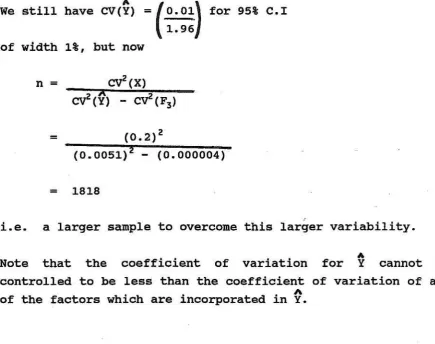
Suppose instead that we wish to estimate the average speed in a

different month, but must sample in the current month only. We

presume there is a factor, F3, available to convert current month

speeds to this other month's speeds, and let us suppose that the

source that gives this F3 value states that CV(F3) = 0.002, which

takes into account that (in the data they studied) the

relationship between months was not exact, the factor being

A

We still have CV(Y) = for 95% C.1

of width l%, but now

i.e. a larger sample to overcome this larber variability.

A

Note that the coefficient of variation for

Y

controlled to be less than the coefficient of variation of any

A

of the factors which are incorporated in Y.

3. STUDIES OF TOTAL VEHICLE FLOWS FROM COUNTS

(A) TO DETERMINE AADT TO A GIVEN ACCURACY

Suppose we are counting the flow along a road for 16 hours each

day, and wish to know how many days we need to count to obtain

24 hours AADT to within 1%.

Table 4 of Appendix D14 of TAM (March 1985 update) provides 'M-

factors' by road type which factor 16 hour counts in stated

months to 24 hour AADT, giving associated CV figures which are

all 6$%. Clearly the CV for an AADT estimate based on a single

count is bound to be greater than 6 % % . Our suggested approach

here is to derive separate AADT estimates from several days 16-

h

where Y is our estimate of AADT

nd is the number of 16-hour counts used F, is the M factor, CV(F,) = 0.065

X is our count, subject to measurement error such that

We understand that most of the variation accounted for by CV(F,)

is due to 'site-to-site' variation in the data set from which

the F, factors were derived. However, our view is that 'day-to-

day' (or 'ambient') variation is also included in CV(F,)

.

this portion of variability could be split off then observations

A

on different days would reduce the variance of Y.

Let us therefore split F, into two factors F3 and F4, with F4

having mean unity and merely allowing for ambient variability.

We have _{F, = F3 F4}

We know

&(F,)

C CV'(F~)

+

Suppose that we can split the CV(F,) such that

(this is for illustration only, but represents our current best

We shall proceed by combining the ambient variability (over

days) with the measurement error, and attenuate both by counting

over more than one day.

Recapping, we have

We will assume that all the counts are taken at a similar time

of year, or at least at 'neutral' times of year, such that F3 can

be taken as constant over days:

-

Where F,X = 1 C Xi

--.

and denotes the mean value

of

using sampling theory for variances of sample means.

The values we obtained earlier were

A

Clearly, if we know n, we can determine &(Y)

,

set a value for CV'(+), provided it is greater than CV'(F,) and

determine sample size n,.

A further refinement is that if there are a fixed number of days,

N,,- in the period under review, we can avoid ambient variation,

Cv2(F4)

,

nd

disappear.

More generally, we can multiply this term by the FINITE

POPULATION CORRECTION FACTOR (FPCF) defined as:

FPCF = N,

-

If we sample only one day this term collapses to unity, while if

Hence all cases are covered by

In order to determine sample sizes we solve for nd, so

While, at first sight, this may appear to overcome the

restriction that, for finite nd

this is not the case, since if the above is violated we will

obtain

which is, by definition, impossible.

A

Hence the smallest CV'(Y) can be is, from our earlier guess,

(0.048)'

A

if CV(Y)

-

then SD(Q)

-

A A

and 1.64SD(Y) = 0.0787Y

Hence the smallest 90% confidence interval for Y, true annual

average daily traffic will be

i.e. a 90% confidence interval could not be as accurate as +5%

WORKED EXAMPLE

If the above values for CV(F,), CV(F4) and CV(X) hold true (i.e.

are 0.048, 0.044, and 0.025 respectively) and if there are (Nd=)

30 days in the period on which the F3 factor is to be based, how

big a sample (in terms of number of days sampled) do we need to

take to be 90% sure we know ARDT to within

+

We must start by reviewing our assumptions, the most important

being that the M factor CV (as published in TAM) of 0.065 might

reasonably be split up into 0.044 from not knowing the average

for the survey month exactly from only taking a sample, and 0.048

for the uncertainty in going from this month to an average month

(presumed due to site to site variability in the data sets used

to determine the M factor). Hence if we sample all 30 days of

the month the 0.044 will disappear, and with smaller samples will

be reduced as determined by sampling theory.

To get a 90% C.1 we need Z=1.64, and to be within y10% we need

So a two day count would be needed.

If the question had been to find AADT to within

+

In which case we would need to sample for 19 days.

4. BEFORE AND AFTER STUDIES OF FLOW

An additional problem arises with Before and After studies, in

that secular growth of traffic may occur, by which we mean

traffic growth which would have occurred even in the absence of

the scheme which we may presume to have been implemented between

the 'Before' and 'After' studies. While it is possible to obtain

national average figures for the rate of growth of traffic, the

applicability of these figures to particular sites is, at best,

dubious.

Our proposal here is to use control sites, unaffected (positively

or adversely) by the Scheme. These sites will show what growth

would be expected had the scheme not be implemented. In order

to best choose suitable control sites we would suggest that two

'Before1 surveys are conducted, at a number of sites including

the site of interest. Since we are only measuring flow, these

'surveys' may sometimes only entail inspecting the output from

permanent counters. The subset of sites whose unexplained growth

between the two 'Before' Surveys best matches that of the site

Having made this selection, the variability of growth rates

between sites between the 'Before' and 'After' surveys can be

expected to be at least as great as that observed between the two

'Before' surveys for the selected sites. Let us denote this

variability VAR(F,), with associated coefficient of variation.

Where F, represents the factor to be applied to the site of

interest to take account of secular growth.

In principle, all the other factors discussed in Section 3 as

being relevant to the accuracy of a count at a single point in

time are also relevant here. However, it is clear that we should

avoid the use of such factors wherever possible by sampling at

similar times in both the 'Before' and 'After' surveys. The

simplest case would probably be to sample after one year in

exactly the same month and exactly the same days of the week, and

for exactly the same length of time as in the 'Before' survey.

This leaves only the secular growth factor to take into account.

In this simple case, consider that as in Section 3 we require to

know how many days to sample for, now both before, nb, and after,

na. Suppose we denote the scheme effect as S, which might be a

figure such as 1.2 to denote a 20% increase. We can set out the

situation as follows:-

T&IA&

'

'

In our estimate of S we will have 'Before' and 'After' flow count

(average) measures

fi,

yb

of variation as discussed above

-

where

ya

-

-

na i=l nb i=l

Such that v A R ( ~ ) = VAR(X)/na

and V=($) = VAR(X) /nb

assuming underlying variability has not increased.

The exact way in which sample sizes will be determined will

depend on the question asked. If we are merely required to have

both Before and After samples each to a given accuracy (so as to

spot a scheme effect) then the theory of Section 3 is sufficient.

However, it is often the case that the question is posed in the

form of requiring Before and After sample sizes so as to be a

certain percentage confident that a given sized change will be

detected as statistically significant at a stated significance

level. Note that the practitioner must now supply the

statistician with three percentages:

(i) the confidence level

-

(ii) the percentage change to be spotted

-

(iii) the significance level for the test of difference

-

5%

In technical statistical terms (i) gives the Type 2 error as 10%;

Suppose that the Before and After samples are taken at identical

times of year and on identical days, then there will be no

factors to apply. We will still have F4 for ambient variability,

having mean 1 and some unknown coefficient of variation. In

Section 3 we have used 0.044 for our CV(F4) and we shall use that

again here, purely for illustration.

Our Null Hypothesis will be that there has been no change, i.e.

H,: P, = P,

Let us take measurements, X, before and after and arrive at

-

Sample means, X, and

q,

adequacy of each days measurement in reflecting the true value

for that day, and day to day variation. Since ambient

variability and measurement error are usually taken to be

proportional to mean it follows that if the scheme causes an

increase, then variability in absolute terms will be higher for

the After survey than for the Before survey. The coefficient of

variation will be constant, though.

Setting the problem out formally, let us choose (for

illustration)

Null Hypothesis, Ho:

P,

P,,

Alternative Hypothesis, HI: pa = (1

+

-

Type I Error: Prob

(Jf,

-

>

From the Central Limit Theorem

Skelton (1982) also arrives at this result.

Adding our factors F4 we have

where Z1 and Z2 are the Z values for the Type 1 and Type 2 errors, on one tailed tests, here

to 2.92, and k = 0.1.

- -

Hence VAR(F4Xa

-

-

-

-

-

If we take the accuracy, in terns of CV, to be equal in both the

Before and After surveys, then

We will usually wish to take equal sample sizes, for efficiency,

so we can solve for nd = n, = nb

The test assumes H,: p, = pbr SO we can further simplify

i.e. one should sample for 5 days before and 5 days after.

In this way variance expressions for S could be developed, set

to desired levels and solved for the sample sizes. This will be

greatly facilitated if we can assume sample s m s to be equal in

both the 'Before' and 'After' surveys, i.e. n, = n,. If the

before survey has already been done, the size of the after survey

If other factors, e.g. adjusting for the effects of month (if

both samples cannot be taken in the same month) have to be

included then sample sizes will increase, as in Section 3, and

become infinite if too high an accuracy is required.

5. COUNTING PARTIAL FLOWS

In this section we shall look at the situation where we are only

interested in part of the flow passing a particular site, e.g.

we may be interested only in vehicles with particular origin/

destination characteristics. In this case there will be some

unknown proportion of the flow, P, which we will need to estimate

so as to multiply it by the estimated total flow passing the

site. We may still wish to count for more than one day, in order

to obtain a sufficiently accurate estimate of total flow.

However, the exigencies of carrying out roadside interview

surveys strongly suggests that we should not interview at a given

site on more than one day. This could be very unfortunate for

our sampling, since the OD mix may vary considerably from day to

day.

The best we can probably do is to confine our interest to

specific sorts of days (e.g. 'weekdayst or 'Sundays1) and to

interview accordingly. We will then be in a position to make the

vital assumption that our estimate of P will apply to the total

flow counted. Let p be the true total flow of traffic per day.

Let P be the true proportion of this which has the attribute of

interest (e.g. if for a specific OD pair).

The daily flow of interest = Pp

We can try to get a good estimate of p by surveying over nd days,

and we can try to get a good estimate of P by taking a sample of

size n. The optimal mix of nd and n will depend on the relative

things as how long the interviews each take, and so we cannot

sensibly even give rules of thumb here. We shall merely indicate

the statistical framework involved.

The variance of a sample proportion is given, for the

Hypergeometric distribution as is relevant here with sampling

without replacement, is

A

Here we do not know P, so use our estimate P, and assume that N

is much greater than n.

Our estimate of the flow of interest will be

CV2

(G)

c

-

-

(l-P) (N-n)

+

If we add the complications of possibly wishing to apply a factor

F,, and possibly having a finite number of days Nd to sample

from, we have

6. MEASURING TRAVEL TIMES

The two main methods of measuring journey times are Moving

Observer (MO), and Number Plate Matching (NPM)

.

case, a car or cars are driven along the link(s) of interest and

the journey time noted. Common sense dictates that the MO should

try to travel at the average speed of other vehicles using the

road. This is sometimes difficult and corrections for cars

overtaken or overtaking are available. Experience at Leeds

suggestedthey were beneficial, but did not make much difference.

The question is how many runs should be made to adequately

determine the journey time. Currently, the COBA9 manual offers

such advice.

Statistically, the question revolves around how accurate each MO

measurement is. Experience in Leeds suggested that MO's, at 15

minute intervals were sufficient to give values which followed

NPM results very closely through the morning peak. Since NPM

is much more expensive, it is presumed here that it will be used

only when there are special reasons, such as needing to know the

spread of travel times on a given link. The conduct of NPM

surveys is a specialist issue, complicated

by

how much of the traffic will actually match, and what will be the

extent of spurious matching. The matter will not be further

If we wish to use MO's, but want to survey on several days-sb as

to reduce measurement error and allow for day to day variation,

then the problem is similar to that of Section 3.

If Xi, is the speed measured on day i, and F, is a (dummy) factor

to allow for ambient (day-to-day) variability, then our estimate

of average speed for several days runs is

-

-

n d ~ 4 2 ~ Z

Where CV(F4) represents day to day variability of speeds, and

CV(X) represents measurement error in that the MO estimate will

not equal the actual average speed on that day. Solving for nd

where the denominator will be determined by the desired accuracy

7. ESTIMATING HOURLY TRAFFIC FLOW

In the preceding sections it has been presumed that we have been

dealing with a day's traffic, e.g. what is AADT?, has AADT

changed etc. We may, however, wish to measure flows in

individual hours, and any d a y l s data can obviously be broken down

into shorter intervals. If we are interested in just one hour

each day (e.g. the 'peak1 hour) then we still have a 'days1

problem since we need to decide on how many days to count this

hour. The basic framework is as set out in Section 3, but

clearly the appropriate factors will differ. Our understanding

is that suitable factors are not readily available to

practitioners.

The best data available to us is from Idris (1981) which may be

interpreted as showing that, duringheavilytrafficked hours, the

day to day (non-systematic) coefficient of variation might be

about 0.05. If we continue to assume a coefficient of variation

of our ATC of 0.025, then we have

CV2 (X)

-

&(F4)

-

-

&(F3)

-

Suppose we wish to measure the true underlying hourly flow (say

between 9 and 10 on weekdays in February 1989) Y, to within 5%

with 90% confidence, then

cv2

(G)

-

-

Using the formula from Section 3

So we should count the hour's traffic for 3 days, preferably

chosen randomly from the 20 weekdays in February.

IDRIS, M K (1981) "The collection and interpretation of traffic

flow data with particular reference to West Yorkshire and

Pakistan Traffic Countstf. MSc Thesis, Department of Civil

Engineering, University of Leeds

Skelton, N (1982) "Determining appropriate sample size when two

means are to be compared1I, Transport Engineering and Control,

Data A ~ ~ e n d i c e s

Secular Growth

Local evidence from historic traffic counts may be available

giving year on year growth and associated CV's. Otherwise use

evidence from 18similar11 sites, or published sources eg. TAM

(fairly out of date) or Transportation Statistics.

Roadway manual suggests that CV's associated with secular growth

between two years, n years apart, are

Source: Roadwav Manual

Historic Evidence of Secular Growth

Motor vehicle flow at average point (1977 = 100)

can be disaggregated as:

Built up roads 1982 1983 1984

Trunk 104 106 109

Principal 109 110 109

B roads 116 119 12 6

C roads 12 5 125 125

Source: Transportation Statistics

Conversion Factors (examples)

HOURS FACTOR SD

12-16 HRS 1.160 0.037

12-24 HRS 1.233 0.040

16-24 HRS 1.054 0.012

(conversion weekday to average weekday; Trunk, A, B, C roads)

DAYS TABC SD

Monday

Tuesday

Wednesday

Thursday

(conversion to a

MONTHS

January

February

March

April

May June

July

August

September

October

November

December

neutral month)

MAIN

URBAN

Unless otherwise stated, factors refer to trunk roads.

Other tables of factors are also available.

Kent Traffic Flow Information

Monthly average flow levels, (sd), (CV).

Other information also available from Kent County Councili

i) A road factors with

+

ii) Monthly factors for M/A/B/C in Kent for 1988 with

+

standard deviation

IDRIS (using completely infilled data)

Road Code MON TUES WED THUR

D402N 6642 6705 6944 6928 (mean daily flow)

567 540 636 812 (sd)

(8.5) (8.1) (9.2) (11.7) (CV)

C302S 6121 6274 6369 6285

993 834 737 877

(16.2) (13.3) (11.6) (13.9)