ADAPTIVE CONTROL FOR TWO
COLLABORATIVE ROBOTS
HANDLING AN OBJECT WITHOUT
VELOCITY FEEDBACK
Dr. E. Balasubramanian
Dept. of Mechanical Engineering, Vel Tech Dr. RR & Dr. SR Technical University, Avadi, Chennai
Mr. S. Riyaz Ahammed
Dept. of Mechanical Engineering, Vel Tech Dr. RR & Dr. SR Technical University, Avadi, Chennai
Abstract:
The kinematic and dynamic equations of manipulators as well as rigid object are presented. The system dynamics is obtained by combining the dynamics of manipulators and the object. In order to avoid the problems encountered due to the measurement of velocity signal, an adaptive control without velocity feedback is employed. This will help us to avoid the need for velocity sensors and ultimately reduces the cost. Stability analysis and corresponding simulations are carried out to show the performance of the controller.
Key words: Manipulator; Adaptive control; Lyapunov stability; Regressor. 1. Introduction
A single robot was not able to grasp and move long and heavy objects in a safe manner. Owing to the serial structure of the manipulator, present day robots are called handicapped operators to perform complex assembly tasks. Collaboration between two manipulators has many advantages [1] such as increase load carrying capacity, greater dexterity and manipulability, reducing the need of extra auxiliary equipments. Moving long flexible objects in a desired path and also precise positioning and orienting the objects need a collaborative action between two robot arms. In most of the control algorithms such as Mater/slave approach [2], Hybrid position/force approach [3], adaptive approach [4], [5] and [6], robust approach [7] and [8] of these kinds of systems, it is assumed that the velocity feedback signal is available. However, in some applications it may not be possible to measure the velocity or may not even be desirable to do it. Furthermore, the use of noisy velocity signal in the control algorithm may create instability in the system [9]. In practice, the joint velocity is measured by means of tachometers or by differentiating the position measurements which are obtained from encoders or resolvers. This necessitates an additional sensor which increases the cost and also the velocity signals are contaminated by severe noise [10]. In order to avoid such problems, a controller without velocity feedback is necessary. In this paper adaptive control law [11] without velocity feedback is suggested.
2. System description and dynamic modeling
Two planar rigid manipulators each with three links and revolute joints handling a rigid object is considered during the model development. The kinematic and dynamic relations of manipulators and the object are derived in the following sections.
2.1 Manipulator kinematics
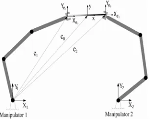
Fig. 1 Two manipulators – object system
The end-effectors position and orientation e1={x1, y1, θ} and e2={x2, y2, θ} are represented with respect to fixed frame X1Y1, respectively. Generally the velocity of end-effector of the manipulator is related to joint velocity of
manipulator through Jacobian Matrix [12]. For the two manipulators, the end-effector velocities 1
e and 2
e and
manipulator joint velocities 1
q and 2
q are related through Jacobian matrices J1 and J2 as follows.
(1)
Differentiating (1) gives,
(2)
2.2 Manipulators dynamics:
The general manipulator dynamic equation is given by [12]
Where i=1, 2 (3)
(3)
For the two manipulators in an assembled form can be written as,
(4)
(4)
Where
2.3 Kinematics of the object
Consider a beam of length L, mass m and the center of object is described by c0={x0, y0, θ}. All the kinematic relations are written with respect to X1Y1 frame.
The left end pose (Position and Orientation) of the beam is given by,
L
L
Tc
e
sin
0
2
cos
2
0
1
(5)
iT i i i i i i i i i i
i
q
q
C
q
q
q
G
q
J
f
M
,
e
J
q
1
e J e J
q 1 1
f
J
G
q
C
q
M
r
r
r
T
2 1
2 1
2 1
2 1
2 1
2 1
2 1
;
; 0
0
;
;
; 0
0
; 0
0
q q q f f f J J J
G G G C C C M M
Mr r r
The right end pose of the beam is given by,
L L Tc e
sin 0
2 cos 2
0
2
(6)Differentiating (5) and (6) results in
0 0 1 0 0 cos 2 1 0 sin 2 0 1 cos 2 1 0 sin 2 0 1 y x L L L L e
rfX
R
e
(7)Differentiating (7) gives,
rfrf
R
X
X
R
e
(8)2.4 Object dynamics:
The Euler dynamic model of the object is given by [1],
0
0
;
0
0
0
;
;
12
0
0
0
0
0
0
)
(
0 02
y
C
G
mg
x
X
mL
m
m
M
f
F
G
X
C
X
M
rd T rd rf rd rd rd rf rd rf rd
(9)
1
cos
2
sin
2
1
cos
2
sin
2
0
1
0
0
1
0
0
0
1
0
0
1
L
L
L
L
F
rd2.5 Combined dynamics:
The dynamic equation of manipulators and object are combined together formulates the system dynamics which is given by,
(10) cs cs rf cs rf
cs X C X G u
M
MoMrd
XrfCoXrfGo Grd uo
Where,
3. Design of controller
The objective of the control law is to move the object in the prescribed trajectory with help of collaborative action between the manipulators. In order to avoid the velocity sensors, control law without velocity feedback is proposed.
Adaptive control law is given by [11],
(11)
Intermediate vectors can be calculated by,
(12)
Adaptive parameter update law is given by,
(13)
Where,
where er= Xrf −Xrfdis the tracking error; cs
is the estimate of cs, then, the parameter error vector can be
defined as cs
~
= cs
−cs; Ya is the regressor matrix, is constant positive definite matrix; , and are
positive constants. It should be noted here that the control law given in (5) and the adaptive parameter cs
can
be found using adaptive law given in (13) do not involve any velocity measurement as feedback. Thus, it avoids the velocity sensors and the controller needs only position measurements.
Substituting (11) into (10) gives,
(14) (14)
Where,
with the introduction of state vector
T
r T T r
T e e
x , , and using (12 ), (13 ) and (14 ) the state space form of
closes loop equation is described by,
(15)
(15)
r T T o T
T
r r
r T T
r T T o
J R u G J R G
R J C R J M R J M J R C
R J M J R M
1 1
0
1 1 1 1 1
1 1
0
1 1 1
;
r
cs rfd rfd rf a
cs Y X X X e
u
2
, ,
r
e
2
2 3er 23er
r
r e
e z
z
Y
aTcs
cs
~
rfd rfd rf cs rfd rf rf cs r
d e C X X X C X X X
C
, ,
(14)
~
2 2
1
r d cs a r cs r cs
r
M
e
C
e
Y
C
e
e
~
cs a r d r
cse C e Y
C C Ax
Where
By arbitrarily selecting the matrices P and Q, one can show that 1/2(PA+ATP) = Q One of the possible choices for the symmetric positive definite matrices P and Q are
Also, the eigen values of P and Q satisfies the following bounds,
(16)
(17)
3.1 Stability analysis:
Stability analysis aims to show that, by properly choosing a Lyapunov function candidate, the proposed control algorithm can accomplish asymptotic tracking performance.
Theorem : The closed-loop system described by (13) and (15) and all the signals are bounded and also limt→∞x = 0, provided the following condition satisfied,
(18)
where λp and λq are the eigen values of P and Q and a function V4(t) is defined in (19). Proof: Consider a Lyapunov function candidate
(19)
Differentiating the above and using (15) yields into
(20)
Then one can
derive the following,
(21) r cs T r r T cs r T r cs r r cs T r r cs T T e C e e M e e M e e M e e PCC x x P x
1
2 1 2 1 0 0 ; 0 0 0 2 0 1 2 1 2 1 2 cs cs cs M C I I I M M A 2
2 0 0
0 0 ; 0 0 1 1 cs cs cs cs cs cs cs cs M M M Q M M M M M P cs T cs TPx x t V ~ ~ 4 2 1 2 1 ) (
cs T cs T cs a r d r cs TTQx x PC C e C e Y x Px
x t V ~ ~ ~ 4 1 2 1 ) ( r d T r r r d T e C e e e PCC x
3Cd
x2
) ( 2 sup 2 3 4 P rf d P t V X C
Px
x
x
T P
2
Qx x x T P Utilizing the property 12 0
r cs cs
r M C e
e , above equation can be written as,
22
1
2
1
x
X
e
C
M
e
e
PCC
x
x
P
x
T T cs r r cs cs r rf
(22)Where, Xrf McsCcs.
Substituting (16), (21) and (22) into (20) yields,
(23)
Where,
and
x
TPC
z
Tand also (13) is used to obtain the above equation. The right hand side of (23) is negative if
rf
X
f > 0, which is true if (18) is satisfied. When q is sufficiently large, (18) is satisfied. By induction
with respect to t, V4 (t) will be decreasing until x =0 which shows that the closed-loop system (15) is
asymptotically stable and hence the given theorem is proved.
4. Simulation results
To illustrate the performance of the suggested controller, simulations are carried out. The parameters of the manipulator and beam, all the initial values are given in [1]. The desired trajectory is chosen as
Xrfd={sinθ,cosθ,0}T. The initial values of cs
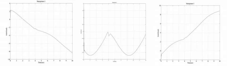
are chosen as =[0.11, 0.06, 6e-3, 6e-3, 0.11, 0.02, 0.073, 0.044, 0.16, 0.11, 0.06, 6e-3, 6e-3, 0.11, 0.02, 0.073, 0.044, 0.16, 0.16, 0.01]T. The initial value of (0) = 0. The control parameters are given as , and and =diag (0.1). Simulation is carried out using Matlab and some of the important results are presented. Fig. 2 and Fig. 3 shows the tracking of the object along X and Y directions and Fig. 4 shows the orientation of the object. Fig. 5 – Fig. 7 shows the joint angular motion of manipulator 1 and Fig. 8 – Fig. 10 shows the joint angular motion of manipulator 2. M1J1 represents the manipulator 1 and joint 1 and M2J2 represents manipulator 2 joint 2. Similarly other manipulators joint angular motions are represented in the captions. It is evident from these results that the desired tracking performance is achieved which validate the controller.
2 ~
2
4(t) 3 C 2 X x z Y 1 f X x
V q d rf T a csT cs rf
rf d
q
rf C X
X f
3 2
5. Conclusion
In this paper an adaptive control scheme without velocity measurement for the case of two manipulators collaboratively handling a rigid object is proposed. The presented control method avoids the need for velocity sensors and ultimately reduces the cost. It also avoids the noisy velocity feedback which may lead to instability of the system. Lyapunov based stability analysis and simulations show that the suggested controller is an effective choice.
References:
[1] B. Esakki, R. B. Bhat and C. Y Su, (2011): Regressor based robust control for collaborative manipulators handling a rigid object, accepted for publication in International Federation of Automatic Control, Milan, Italy
[2] Y. F. Zheng and F. R. Sias, (1986): Two robots arms in assembly, in Proc. IEEE Int. Conf. on Robotics and Autonomous System, pp. 1230-1235.
[3] M. Uchiyama, N. Iwasawa and K. Hakomori, (1987): Hybrid position/force control for coordination of a two arm robot, in Proc. IEEE Int. Conf. on Robotics and Automation, pp. 1242-1247.
[4] Y. R. Hu and A. A. Goldenberg, (1998): An adaptive approach to motion and force control of multiple coordinated robots, in Proc. IEEE Int. Conf. on Robotics and Automation, pp. 1633-1637.
[5] M. W. Walker, D. Kim, and J. Dionise, (1989): Adaptive coordinated motion control of two manipulator arms, in Proc. IEEE Int. Conf. on Robotics and Automation, pp.1084-1090.
[6] B. Yao and M. Tomizuka, (1993): Adaptive coordinated control of multiple manipulators handling a constrained object, in Proc. IEEE Int. Conf. on Robotics and Automation, pp. 624-629.
Fig. 5. M1J1 angle Fig. 6. M1J2 angle Fig. 7. M1J3 angle
[7] I.Uzmaya, R. Burkan and H. Sarikaya, (2004): Application of robust and adaptive control techniques to cooperative manipulation, Control Engineering Practice, vol. 12, pp. 139-148,
[8] W. Gueaieb, F. Karray and S. Al-Sharhan, (2007): A Robust hybrid intelligent position/force control scheme for cooperative manipulators, IEEE/ASME Transactions on Mechatronics, vol. 12, (2), pp.109-125.
[9] J. H. Yang, (1999): Adaptive Tracking Control for Manipulators with Only Position Feedback, in Proc. IEEE Canadian Conf. on Electrical and Computer Engineering, pp. 1740-1745.
[10] M. A. Arteaga, (2003): Robot control and parameter estimation with only joint position measurements, Automatica, vol. 39 (1), pp. 67-73.
[11] C. Y. Su and Y. Stepanenko, (1998): Redesign of hybrid adaptive/robust motion control of rigid-link electrically-driven robot manipulators, IEEE Transactions on Robotics and Automation, vol. 14 (4), pp. 6.