A comparison and evaluation of risk and uncertainty techniques for capital projects in the public sector

Lincoln

University

Digital

Thesis

Copyright

Statement

The

digital

copy

of

this

thesis

is

protected

by

the

Copyright

Act

1994

(New

Zealand).

This

thesis

may

be

consulted

by

you,

provided

you

comply

with

the

provisions

of

the

Act

and

the

following

conditions

of

use:



you

will

use

the

copy

only

for

the

purposes

of

research

or

private

study



_you

_will

_recognise

_the

_author's

_right

_to

_be

_identified

_as

_the

_author

_of

_the

_thesis

_and

due

acknowledgement

will

be

made

to

the

author

where

appropriate



_you

_will

_obtain

_the

_author's

_permission

_before

_publishing

_any

_material

_from

_the

thesis.

A COMPARISON AND EVALUATION Of . RISK AND UNCERTAINTY TECHNIQUES FOR CAPITAL PROJECTS IN THE PUBLIC SECTOR.

A thesis

submitted in partial fulfilment of the requirements for the Degree

of

Master of Agricultural Science in the

University of Canterbury

by

Brian A. 8el1

Lincoln College 1975

, I

>-I·:;

ABSTRHCT

.,-.

The basic problem facing decision makers is the

allocation of scarce resources among comp8ting users, Such

decisions mads are usually in the face of an essentially

unknown future environment~ This thesis is concerned with

making good decisions under uncertainty in relation to

public investment proposals in New Zealand agriculture.

A case is put for the evaluation of risk and uncertainty

in agricultural projects, but on a review of evaluation techniques in use it is found that many deficiencies exist. In a search for a practical solution t.o the risk analysis

problem it is shown that decision theory shows very little

promise. Rather the solution is to r"ake the risk and uncertainty explicit by presenting the present value in

terms of its probability distribution. Two methods are

discussed, they are Analytical Techniques and Monte Carlo Methods.

The analytical technique is developed through the use of probability calculus. Techniques evolve from being able

to calculate the variance of simple summed random variables

to handling complex combinations of products of random variables using Taylor's Approximation. Incorporated in

the analysis are discussions on subjective probability distributions, forecasting techniques and corrulation analysis. It is shown that the shape of the probability

the variables relate to each other both within and between

periods. Earlier criticisms of~traditional techniques of

handling risk and uncertainty are overcome. In the

analytical technique judgment is applied to the underlying assumptions in the project rather than to the results of the analysis. The variability of the project is measured

by a single overall indicator (the variance), not by a number of criteria. The technique allows for interaction

between the variables which make up the project. A quantitative assessment of risk is made rather than

quali tative statements and lastly tile basic fral~,ework is

laid for consistent analysis project to project and analyst

to analyst.

Monte Carlo Simulation offers two major advantages

over analytical methods. These are firstly, all the characteristics of the probability distribution of the

variables can be simulated and secondly the dynamic aspects

of project development can be incorporated into the

analysis. There are, however, cert8in drawbacks to

implementation. The major disadvantage is the time required to build a simulation model. The task of

developing a general package was found to be beyond the

scope of this thesis. The main problem encountered was in defining and incorporating the dependency relationships

between variables.

A rural water supply scheme 1s analys8d und8r several

of each method. It is cqncluded that the analytical

technique incorporating Taylorf~ approximation shows the

r

I

CONTENTS

,,','

CHAPTER PAGE

I. INTRODUCTION 1

1.1 Problem Formulation 1

102 Background 1

1.3 Outline of the Study 4

II. THE EVALUATION OF RISK AND UNCERTAINTY IN

THE PUBLIC SECTOR : A REVIEW OF LITERATURE. 5

2., Introduction 5

2.2 Cost Benefit Analysis and Risk and

Uncertainty. 5

2.3 Uncertainty and the Evaluation of

Public Investment Decisions. 7

2.4 Traditional Methods of Handling Risk

and Uncertainty. 12

2.5 The Methods Used in New Zealand

Agriculture. 16

2.6 Theoretical Considerations. 23

2.7 SLlmmary 0 31

III. THE ANALYTICAL METHOD. 32

301 Develo'pment of the Mathematical Model. 32

3.2 Estimating Cash Flow Elements. 45

- 3.3 Correlation. 55

IV. Srr~ULATIONo

4.1 Introduction.

4~2 Simulation in Perspectiveo

4.3 Monte Carlo Methods.

4.4 The Structure and Properties of a Simulated Agricultural Project.

405 Application of Simulation to Capital

Investments. 4.6 Summary.

V. COMPARISON OF THE MODELS. 5.1 Introduction.

5.2 The Models.

5.3 The Models Compared~

5.4 Conclusions.

5.5 In Depth Analysis Using ANWA.

65 65 66

68

69

71

87

88

88

89

99

103 105

5.6 Possible Improvements to the ANWA Pr.ogram. 106

VI. CONCLUSIONS AND REcor~r~ENDATIONS. 108

6.1 The Problems of Implementing Risk Analysis. 108

6.2 The Advantages of RisK Analysis. 109

6.3 Implementation. 110

ACKNOWLEDGMENTS REFERENCES APPENDICES

112

LIST

or

TABLE PAGE

1. InvG~tigations carried out by the Department of

Agrtculture into proposed water resource projects. 2

2. Basic forecasting techniques. 46

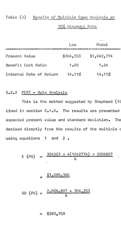
3. Re8ultsof mu~tiple case analysis. 90

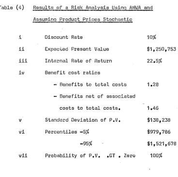
4. Results of a risk analysis using ANWA and assuming

products prices stochastic. 95

5. Results of a risk analysis using simulated samples frool the mUltivariate normal distribution •. '

Assuming product prices stochastic. 96

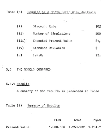
6. Results of a Monte Caro risk analysis. 99

7. Summary of results. 99

8. Computer time required by each model

.

.

102

9. The effect on the standard deviation of increasing

..

the number of variables within the risk analysis. 105

-;,'

10. Product price distributions. 14~

11. Distributions of productivity levels. 141

12. Total stock increaseso 14'

13. Percentage distribution of total stock increases OVE>r

time. 1 "."

14. Stock increases. 150

15. The first derivatives of the price analysis. 1~'l.

.,

!

i

LIST OF FIGURES

FIGURES PAGE

1. Utility functions. ₂₇

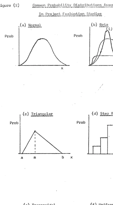
2. Common probability distributions assumed in project

evaluation studies. ₅₁

3. A Monte Carlo computer algorithm. ₇₄

4. Time growth in a probability distribution. ₇₆

5. Monte Carlo Simulation using the multivariate

normal distribution. ₈₀

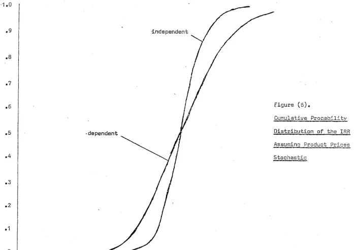
6. Cumulative probability distribution of the I.R.R.

APPENDICES .{'

PAGE

I Economic Report on the Tuapeka Rural Water Scheme 122

II

Variables 145

III

IV Disaggregation of the Cash Flows to obtain the

First Derivatives 160

v

Listing of program and input data for the full analysis.

VI ANWA - Layout for card input 178

VII MVSM - Listing of program, \nput data and output 181

VIII TUAP - Listing of program, input data and output 192

1.

CHf.IPTER I

INTRODUCTION

1.1 PROBLEM FORMULATION

The basic problem facing decision makers is the·

allocation 6f scarce resources among competing users. Such

deoisions made are usually in the face of an essentially unknown future environment. This thesis is. concerned with making good decisions under unoertainty in relation to

,

public illvestment proposals in New Zealand agriculture.

1.2 BACKGROUND

During the late 1950's and early 1960's the Farm Management and Economios Section, of the New Zealand

Department of Agriculture, was increasingly oalleD upon to oarry out land utilization and farm management surveys. The purpose of these was to assess the potential produotion inoreases arising from developments in farm water supply, irrigation,· land reclamation and farm improvement sohemes

(see Table I).

E!.1'.9r:~~ure into<..Erop.9.~8.~at£~C}~

?roj8c~~

Year ended Water Corrservation

31st March Irrigation Supply Drainage

&

River Control

1952 1

1953

1954 1

1955 1

1956 1

1957 2 3

1958 2 1

1959 1

1960 7 2

1961 1

1962 1

1963 2 2

1964 1 2

1965 1 3

1966 1 7

1967 6 2 2

1968 6 6 4

1969 4 5 1

1970 4 8 4

1971 2 8 6

1972 2 10 10

1973 2 10 7

Source: Resource Section', Economics Division,

M.A.F.

Palmerston North

Total 1 1 1 1 5 3 1 9 1 1 4 3 4 8 10 16 10 16 16 22 19

1 The off-farm capital costs of these projects range from 52000 to over $15,000,000 with an average of $770,000.

2,.

In the early reports the accounting rat.e of return was used as the dFJcision crited.ol1o " Ciscounting and the use of

present values was first incorporated in 1964. By 1966 the

techniques used in the analysis had been refined considerably and procedures developed were adopted nationally. The term Cost Benefit Analysis was first applied to the reports in 1967, although they were still stricUy project appraisals at that time. Sensitivity analysis of uncertain parameters such as product prices, scheme capital costs and project life were included in the analysis of some schemes.

With the Pormation of the Economics Division in the

latter half of 1970, a Resource Section9 within the Division

was set up in Palmerston North. Its major responsibility was

to investigate and prep8re economic ~eports evaluating

agricultural projects from the national point of view. Thus

for the first time project evaluation reports o~iginated

from the one centre. One result was that reports became

consistent in analysis and layout. f

r: :: :~. . --'

In 1971, by directive of Treasury, a ten percent

weighting for overseas funds content was added to benefits and costs.

Also at this time the PERT-Beta technique for risk analysis was introduced into the analysis. Subsequently this aspect has been questioned both on theoretical issues and from

the practical conclusions that were being drawil from it. The

103 OUTLINE OF THE STUDY

The study proceeds in the following way. In Chapter II

a case is presented for carrying out risk analysis in the public sector, present evaluation techniques are critically

examined and it is concluded that techniques which incorporate probability analysis show the most promise for improving

evaluation techniques. Chapter III outlines in some detail

Analytical Techniques for risk analysis which are bas~d on

probability calculus and subjective estimating procedures.

Chapter IV introduces the Monte Carlo Simulation technique for risi< analysis which although having several advantages

over analytical techniques also has ~ajor limitations to

implementacion. In Chapter V a particular project ie analysed

using the previously discussed t~aditional methods, analytical

techniques and Monta Carlo methods. Chapter VI_presents the conclusions to the study and recommendations as to the

CHAPTER II

THE EVALUATION OF RISK AND UNCERTAINTY IN THE PUBLIC SECTOR: A REVIEW OF LITERATURE

2.1 INTRODUCTION

This chapter proceeds as follows:

1. The concepts of Cost Benefit Analysis and risk and uncertainty are introduced. 2. The relevance of under-taking risk and uncertainty analysis in the evaluation of investment projects in the public sector is discuBsed and justified. 3. Traditional methods of handling risk and uncertainty in pruject evaluation are reviewed. 40 The methods used by the Economics Division M.A.F. are reviewed

and evaluated. 5. The decision theory approac~ to risk and

uncertainty is discussed, and the concepts of utility analysis and the maximisation of expected utility are introduced.

2.2 COST BENEFIT ANALYSIS AND RISK AND UNCERTAINTY

The basic idea behind Cost Benefit Analysis is to decide whether a project involving public expenditure has a positive or negative effect on society. This implies the

evaluation of all the relevant costs and benefits. It involves the welding together of a variety of traditional areas of

Although the origins of Cost Benefit Analysis go back

to Dupuit (11]/14) the practical aR.plication of the theory to

public investment did not occur until the 1950's. Since then there has been a flood of literature on the theoretical and practical problems associated with the technique. Two

widely acknowledged general surveys of the literature are those of Prest and Turvey (1965) and Henderson (1961).

Welfare aspects are well covered in Krutilla (1961), and Winch

(1971), while a review of investment Pila1ysis in the public setting may be found in Muthoo (1972) with applications in

Turvey (1968). Practical problems and applications are high-lighted in Mishan (1971) and Oasgupta and Pearce (1972).

Also, Little and Mirrlees (1969, 197~) have made a major

contribution to social cost benefit analysis in developing

countries, particularly in the field of shadow pricing.

Major problem areas in Cost Benefit Analysis include

the measurement of costs and benefits, external effects, the choice of investment criteria and the measurement of

uncertaintYe As previously indicated this thesis addresses

itself only to the latter problem: that of risk and

uncertainty. Ho\~ever, before delving into this, it is

important that the terms risk and uncertainty be defined for

the purpose of this thesis.

2.2.1 .Q§!initions I

Henderson (1968, p 138) writeA as follo~s:

"Risk is defined as a situation in which the outcome is

uncertain, but the probability distribution of outcomes is knolJJn with certainty.· This may be called .a.ctuarial risk2 •

.... "'~..l.._~~_4~ _ _ _ _ _ _ _ _ _ _ _ _ _ _ _ _ _ _ _ _ _

'" I 0

At thB other. 8xtremB, wh81~8 nothing ltlhatov8r is klllJlJJn alJQut

the probability distribution lJJr) h.B.ve the case of .EL!.;"S.q,

AJ. though most actlJal situations fall strictly

under neither heading, they may quite often approximate more

or le88 closely to one or the other, and be b~8at.8d

accordingly~ Tho intermediate cases which are not close to

one extreme or the other can be described as situations of

!!.O..Certai.!Jll" with no qualifying adjectiv~. Tho dO.9-£.8B. of

actuarial risk may be represented by the variance or the

standard deviation of the probabiJ.:i. ty distributi.on

0"

"Risk¥, choice prevails when a decision mal<er has to cho080 between al tornatives, some or all of lJJhich have consequences that are not certain and can only he described

in terms of a probability distributionll (Dillon, 1971, p 4).

From these two quotations it can be ssen that

Henderson's "uncertainty" is synonymous \I)i th Dillon's "risky

choice". In this thesis the terms risk and uncertainty will be used to describe random variables that fall within the

bOllnds of Dillon's "risky choice". That is, random variables

that may be described in terms of probability distributions.

1---:-:-:,:-:<·-::-:::

2.3 UNCERTAINTY AND THE EVALUATION

or

In the private sector managers behave as risk averters and generally use interest rates that are much higher than

would be the case if costs and returns were known with

0,.

decision makars in the public sector should follow suit and

make allowance for risk and unc8)~tainty ill pubLic investment

projects. Current practice in New Zealand is to make

allOl~arlces for risk and uncertainty. Battersby and Smallbone

(1970) considered that projects in the public sector are often faced with the same uncertainties as those in the private sector and therefore the discount rate should reflect this.

They did however 1I ••• acknowledge the fact that by anci large

Government investment is relat.tvely low riskDII In recommending

a ten percent discount rate they took both ti~e preference and

uncertainty into account. The rate is based on the opportunity cost of capital in the private sector, but is reduced slightly to acknowledge the lower risk of Government projects. 3

This view that risk and uncertainty should be taken into account in the public sector is supported by Hirshleifer (1963 , 1966). He argues that the same rate should be u-sed in the

private sector - to do otherwise would be an argument for the

"second bestll (Hirshleifer, 1966, p270). In other words, if a

lower interest rate was used in the public sector, projects would be -accepted that would otherwise have been rejected by the private sector. This would result in an inefficient use

of capital.

On the other hand Arrow and Lind (1970) reject this view. They show that .when the risks associated with a public investment are pUblicly borne, the total cost of

risk-bearing is insignificant and therefore Government should

---

..

ignore uncertainty in evaluating pub1ic investments.

Similarly, the choice of discount rate should be independent

of considerations of risk~ ThiG conclusion is reached, not

because Government can pool investm8nts, -but because

Govern-ment con distribute the risk among a large number of people. Their conclusions are conditional on tha investment being

independent of other components of national i~come. However,

if some Government investments are interrelated they should be evaluated as a "package". /\fter such grouping they

contended that there would still be a relatively large number of essentially independent projects.

However~ there are several bases where Arrow and Lind's

general conclusions do not hold.

The first concerns the situation where a substantial

proportion of the benefits and costs accrue directly to individualso In this case, as the individuals incur the

attendant cost of risk taking, it is appropriate to take risk

into account.

An example of such a situation could be an irrigation

scheme or other land bettermont proposal where the farmer bears a major proportion of the costs and benefits. The major sources of uncertainty to the farmer may be listed .under the

following headings:

(a) Technical This includes such factors as the

design failure of the project, the failure to reach estimated physical production levels and the performance of new crops.

The main uncertainties are the

(c) Personal

~~~-- These factors 81'8 main} y psychological..

The farmer is concernod wi th prob}[ml~) such as his own 8bili ty

to adapt to change, his life expectancy and the ages and

attitudes of his childrBn. 4

However, all these uncertainties will not accrue solely

to the proj~ct. Past Bxperience has shown that Government is

willing to come to the aid of farmers under adverso technical and economic conditions (Frampton, 1971, pp 5-10).

From the farmers' point of view the unc8rtaint~ dU8 to

the project is almost entirely personal. However, technical

and economic uncertainties are present whether the project is implJmentBd or not and these can also be modified by the

Government's actions. To the farmer, the uncertainty as to

his own pe~formance is paramount. This is borne out by the

reluctance of many farmers to vote in favour of schemes even though the monetary returns appear very favourable. They are

uncertain as to whether they can cope.

Frengley (1972) points out that these social conse-quences are rarely considered. The analyses generally assume

that an increase in monetary benefits leads to an increase in

the welfare of the individual. However, the disutility of adjusting to a new system, of the probable loss of leisure

time and the additional worry due to increased capital and

labour requirements are major considerations to the farmer.

4 _Th~s . _{concern with the ability to cope with change is by no}

means peculiar to farmers. Schon (1971) maintains it is an increasing phenomenon of our times.

_.-11~

It is important that the analyst be aware of these particular

uncertain ties and mudi fy his expectations of tho far'lilers!

future actions accordingly.

The second case where a risk analysis should bo carried on a public project occurs when regional considerations are

important. ror example, the failure of a largo projoct could

haVB particularly damaging effects within a region.

The third case for a risk analysis in public investment

occurs when a particular project or package of project~ (as

defined earlier) is large when compared with national income. This is not such a relevant argument in New Zealand's

situation but is appropriate where a small country depends

solely on a single large investment. ~owev8r, of considerable

importance -1;0 New Zealand is the generally wide fluctt~.3tions

in the balance of payments. It i~ a widely held view that

attempts should be made to reduce these fluctuations. This

implies selecting investment projects that take into account

the variance of Present Value where overseas funds are

involved. This is particularly im~ortant to agriculture as

over 70 ~ercent of New Zealand's export receipts still come

from meat, wool and dairy produce.

A final reason for taking risk and uncertainty into account stems from the political nature of decision making.

Politicians generally have the final say in choosing large scale investment projects, and because they do not wish to be

associated with failure, it is likely that the risk and

uncertainty aspects of projects pInyan important raID in their

120

It appGars from the above discussion that there is still a case for evuluating Government projects in ttle agricultural

sector for risk and unc~rtainty. Briefly, main reasons are

that individuals often bear a large proportion of the costs and

benefits of agricultural projects, and that regional and political considerations can be important.

The questiun now remains of how the analysis should be

carried out. It is my contention that present methods of dealing witl, risk and uncertainty in the New Zealand

agricul-tural sector are somewhat arbitrary, generally inconsistent and

at best confusing. These methods will now b~ reviewed and

practical alternatives suggested and evaluated.

2.4 TRADITIONAL METHODS FOR HANDLING RISK AND UNCERTAINTY

Traditional methods have generally fallen short of their

objectives. This section briefly reviews some of the more common traditional methods and shows where they are deficient.

The basis of the problem lies with the data estimation. It is

this point .which is taken up first. 2.4.1 Data Estimation

The estimation of future costs and revenues are the most difficult aspects of' project evaluation. Techniques used

for estimation are very diverse. They range from being

care-fully considored computations to off-hand approximations, little better than guess work.

The bosic problem is that most prospective projects for

dealing with a situation in hlhich a large body of relevant data

allows us to predict the degree

or

is seldom relevant data that may be used directly. Thus the estimates or forecasts are often subjectj.ve evaluations

based on incomplete evidence indicating what the futUre might hold ..

The methods used depend on the data handling facilities,

analysis skills, types of information1 and the time and money

available for the estimation. A review of estimation procedures in comman use is given in Chapter 3 under Forecasting Techniques,

Having estimated values for the elements in the analysis, the problem now arises as to how they should be combined to

evaluate a project. Klausner (1968) provides a very good review

of the tra~itional techniques. These include:

2.L~.2. The lissumed CertaintY_.BE.BrJach

Assumed Certainty is the most common method used in project evaluation. Single estimates are used to determine the

outcome of the investment. These best estimates are generally

modal or most likely values and t~erefore when combined do not

give the expected value of the project5o The major advantage of

this approach is that it does not require the analyst to make detailed estimates of cash flows. Indeed the popularity of

discounting procedures stems from this fact. However, by itself

the assumed certainty approach is not very helpful as it does not

explicitly consider the uncertainty of the investmBnto

5 _{Wagner (1969, p655) shows that given a non-linear function}

f(x 1 ••• xn) of random variables x1'.' xn it is usually erroneous

to assume that E

[f(X

fallacy of using averages.

I • -.. •• ~ -:-.' ';;-,'

~·_v:v:-:..:·.-~-;-:.

'14 ..

USB of the payback period method implies a desire for

.;,..

early rather than late returns. Its major drawback is that

it does not take into aCGount the effect of cash flow

patterns and length of project lifo. For these reasons it must be discarded.

The conservative adjustment approach alters costs up

and benefits down to allow for uncertainty. The main prob18m~

that occur with this method are that adjustments are entirely subjective, possibly inconsistent and when combined

statistically unsound. It becomes very difficult for the

d8cision maker to interpret the adjustments. There is also a very small likelihood that all the cons8rvative estimates

will occur together. This leads to what Klausner calls an

"overkill" effect. At best, this obscures the investment picture and at worst gives an entirely false impression.

2.4.5 Sensi.livity Analysis

The sensitivity analysis method usually consists of varying within a range, on a percentag8 basis, the uncertain

elements, one at a time. It has the good offect of

high-lighting the relative importance of accurately estimating each

element~ For this reason it may be useful in a post analysis

stage to isolate one or two critical elements. However, as a

method of analysis by itself it lacks conciseness, and

comprehensiveness. A major problem arises because it does not

usually give an estimate of the prob~bility that a percentage

15.

distribution of B variablo is considered in deciding the range

IlJi thin which the sensitivity analysis is to be conducted, then

the more sophisticated method to be discussed later can be

appli8d~

2 .4. 6 n2-v~Js"_A~.~:!.~>,t~.sL_P~~~D,,:t..B a ~1:.

Raising the minimum acceptable rate of return is basically

the same as usinO the assumed certainty method except that it

adjusts the discount rate up as the risk and uncertainty of a

project increases. As with the payback period method this

technique discriminates against projects with a long life. Its

major drawback however1 is that it becomes subjective in

deciding what leval the discount rate should be raised or lowered

for differont levels of risk between projects. The arguments for

using this ~ethod are essentially circular. It is assumed that

the riskiness of the project is k~own so that it can be classed

with similar ventures which pay a known market pr.ice for capital.

As Van Horne (1972), and others PQint out it is the risk-free

rate (the time value of money) that should be used as the discount

rate.

2 • 4 • 7 frJ!1JJ-.DS.LJ~l j:}.

e

In running multiple cases several or all the elements are changed at once. The most usual case is evaluating the project

with all elements first at optimistic levels, then at most likely

levels and finally at pessimistic levels. However, knowing the extreme ranQe that the project can take does not provide the

decision maker with much useful information unless he knows the probability of occurrence. Even then the probability of all the

values being high or low lulll be extremely small. This method is

16.

2.5 THE METHODS USED IN NEW ZEALAND AGRICULTURE

2 • 5 • 1 .t;.9_ [) tJ~,~~e f !.t_0~~L~

Ward (1964) was the first to advocate ths use of Cost

Benefit Analysis in New Zealand. During the mid 1960's

New Zealand had just emerged from a period of slow growth in

the 1950's ~nd early 19601_{s. Ths prevailing mood was orientated}

towards economic growth and Ward saw the need for a systematic mothod for the evaluation of the large number of investment

projects set before Government. His concern was that there should be a common basis of comparison (between project reports)' so that the relative merits of indi0idual projects could be

6 reviewed in a more consistently objective manner •

Since then the technique of project evaluation has been

disseminated through the universities7 to Government and Local Body Agencies which are largely responsible for implementing the

technique.

Traditionally project evaluation procedures have failed

to deal adequately with the risk and uncertainty problem.

6 _{The Maraetai Study (Ward ~~. 1965) served as an}

illustration of the suggested methodology.

7 _{Jensen (1968) edited the proceedings of a seminar designed}

In a review of agricultural and forestry evaluation studies in NRbJ Zealand Orsman and Johnso

_l1

" 8 report included a full scale analysis of uncertainty.

Most authors approached the problem in a qualitative way. Estimation of data proved to be the most difficult problem.

For example Chisholm (1962) emphasised the difficulties of estimating physical input-output relationships, and predicting

resource costs and product prices up to 50 years ahead.

The methods used for dealing with risk and uncertainty

may be summarised under the following headings: 2.5.3 "l,he M"sthods

(a) £2.Q..seIvative Adjustments tn Data,. Generally when

conservative adjustments to data are made, cost type elements

are adjusted up and revenue type elem8nt~ are adjusted down

(TlJJOmey, 1955).

(b) ~ensitivity Analysis. Where it is felt that a

particular element has a critical effect on the profitability

of a project then a sensitivity analysis is carried out. There are many examples including:- capital costs (van Asch,

1970), project life (Butler, 1969), area developed (Bryant,

1972) and the discount rate (Plunket, 1964).

(c) ~ltiple Cases. The usual situation is to analyse

the project at three levels using pessimistic, most likely and

optimistic estimates of elements. This method forms the basis of the present technique used by the Resource Economic

Section of the Ministry of Agriculture (Forbes, 1973).

---"---"8

(d) BisJ,~<~(l9j"'Jo~")J;l:;!-! 0J-_sS9l:!nL~.E.t~.4 The ten percent discount rete LJSG:cJ by nIl Government Departm8nts in New

Zealand is risk adjusted& In 8 Tro8sury par1GI: Battersby and

Smallbone (1970) stated that "~e.Public investment projects

are often subject to the same uncertainties as arB projects in the private sector and the discuunt rate used should

18 ..

reflect this fSC·t.1I Th(3 authors considered that the "risk

free" rate ~Ja8 about 6.5 percent. This was based on the Cost

of Borrowing approach. However, in their view, the Opportunity

Cost of Capital (12-15 percent) provided a more acceptable

basis for choosing the rate. The ten percent rate finally

suggested, was a valLJ(~ judgment, in part to "acknowledge the

fact that by and large Government investment is relatively low

risk." ••• that is, lowc~ than the risks in the private sector.

(e) ~inati~2f Above Me~b~~. Often aspects of

the above four methods will be incorporated in ~he one analysis.

The result being that decision makers are not faced with a consistent set of analyses of different projects.

To use a risk adjusted discount rate and then allow for risk through the use of variance is double counting and there-fore tends to reject more projects than is appropriate.

Also risk adjusted discount rates imply that' all

variables in the present value equation are subject to the same

degree of risk, which is proportionate to time - an invalid argument.

(f) .0.!l..I.X}~52,~ti.9ll_"t.9~~Ru.!.~,. There has besn one detailed analysis of uncertainty in project evaluation in

Dev(-3lopfTIsnt" (1970), a ninistry of WOI'I~s Public8 t,ion 0 In

Appendix XI of' the report Vign8Llx_ de:::;cribcs the uncertainty analysis. It is based on tho concopt of Range (Vignaux, 1966). Range gives the simplest estimate of tho standard deviation

for normal popUlations where Range equals the High minuB the

Low estimate (Snedecor, 1961). A major assumption in the

analysis is that the ranges of different variables are inde-pendently normal. Given this assumption Vignaux calculates

the total uncertainty by taking the square root of the sum of squared Ranges. Probability statements are then made by an

appeal to the Central Limit Theorem.

I t is stated in the report that the major uncertainty Jiss in price trends for Agriclll ture and Forestry. Thus, for

prices the Range is cGlculated by taking an wpward trend of

o.~ percent per year and an equal downward trend. Without

giving a detailed criticism of the analysis it ~s fair to say

that the analysis contains heroic assumptions about the

independence of variables. There is also a conservative bias

i~ a number of the estimates and the mathematics and use of

Range to estimate the standard deviation is open to question

(Snedecar, 1961, P 110). However, to my knowledge, the report

represents the first serious attempt at a full uncertainty analysis in New Zealand and must be commended for this.

2.5.4 Deficiencies of Trad:iJi9.,n.al r~ethod~.

Klausner op.cit. ably sums up the deficiencies of these traditional methods.

"a. Judgment is usually applj F3d to t.he I'8sul La of the

analysis rather than to the underlying assumptions.

f

-'<'--"-.->-",-;'.-

1:-:::-:,-:-:-:-:-:-:--F.4;i~~~~@}~

i

1'_:::.---b. Thel.'G is no oVEJrall indicatol.' of outcome variability _ _ "!Mr _ _ _

genSI'atc3u.

"

c~ There is no accounting for investment element inteI'~

action.,

d. These methods result in a qualitativo !lfesl" rather than a quantitative assessment of risk.

8 0 They du not provide a consistent analysis framework

either project to project or individual to individual."

In an attempt to overcome these types of criticism

ShepherJ (1970) introduced the so-called PERT- 8eta9 method for handling risk and uncertainty into the evaluation of

projects carried out by the Resource Section.

The procedure involves the calculation of the mean and

standard deviation of the project's present value. This is carried out as follows:

Firstly the project is analysed at three separate levels of prices. 10 These prices correspond to pessimistic, most

likely and optimistic levels. It is assumed that there is only

a 0.05 probability of the pessimistic or optimistic levels being exceeded.

9 _{PERT - Program Evaluation and Review Technique. See}

Malcolm ~~ ale (1959) for details of the techniqueJ

Moder and Rodgers (1968) for practical applications and the Federal Electric Corp. (1967) for a programmed introduction to

the method.

10 _{Uncertainty is evaluated for product prices only.}

The three nGt cash flows(pessimistic, most likely and

optimistic) are then discoL/nt8ds~parat81y using a ten percent

social discount rate and the expected present value and standard deviation are calculated as follows:

E( PV) ::: ~.!L±.2 _{• •}

b

•

•

•

'S.D~ ::::

6-

•

•

where a :::: the present value of the pessimistic net cash flow.

m ::: the present value of the most likely net cash flow.

b ::: the present value of the optimistic net cash flow.

Equation (2) infers that the range given by the optimistic

minus the pessimistic net cash flows covers 99 percent of the

total range (or six standard deviatio~s). Dividing the range

by six giv£s the value for one standard deviation,

Thus, assuming that the prasent value is approximately

normally distributed, equation (2) may be interp~eted as stating

that there is a 63 percent chance that the actual present value will lie within plus or minus one standard deviation of the

calculated mean.

However, use of equation (2) relies on a very dubious

assumption; namely that the prices used in the calculation are

fully dependent. That is, they have a correlation coefficient of one. This means that if one price is at its optimistic

level then all other prices are assumed to be at optimistic

levels - and moreover for the whole of the project life.

If, on the other hand, it is assumed that all the prices are strictly independent, th8n equation (2) becomes an invalid

ten independent variablsG in the project e8ch with a

probability of D.DS of being optimistic or pessimistic, then

the rJJ:Ohi..1bili t.y that they liJould all be optimistic is (0.05). 10

°IOh' _{l8 ,18} • 10-'14 _{• The ran~)f.J that this covers" would be}

apPl'oxim-ately 208tand~rd deviations. Therefore dividing the range

by 20 would give a more meaningful estimate of the standard

d . t' "sv:Joa .olon •. Equation 11 (2) would then

become:-S.D. :::: b -₂₀ a • • • • • • • • 0 • 0 (3)

Use of equation (3) as a valid criterion for judging

the uncertainty of projects rests on the assumptions that prices are strictly independent and that they remain constant over the life of the project.

As these assumptions are not acceptab~18 the PERT - Beta

Technique was discarded in 1972.

The method now used by the Resource Econo~ics Section

is a less positive explanation of tho risk and uncertainty

associated with projects. It is based on the three product prjce levels which give a range or space wherein the results

may lie. It is left to the decision maker to define at what

point within the range the result should lie (Orsman and

Johnson, 1973 pp 22-23). However, the analyses stiil incorporate all the dubious points of the traditional methods.

The techniques may incorporate biased collection of

data. The uncertainty issue is still confused by the use of different combinations of sensitivity analysis. Double

11 This was pointed out by La Page (1973) in an Economics

Division internal discussion pCJper.

countin'] for :risk Hnd uncFJI'tainty is pref30nt due to the risk

adjusted discount rate and the uso of conservative data

adjustmsntso Finally no probability estimate i~ placed on the

range Of the present valuGo While these inconsistencies are

present it cannot bo hoped to make good decisions when

comparing a number of projects or in fact judging whether a project passes a certain profitability criteriono

In order to eliminate the above inconsistencies and deficiencies a return must be made to basic theoretical decision making. In this next section the decision theory

approaci I to risk and uncertainty is discussed 0 I t will be

fpund to lead to utility analysis and the maximisation of expected utility.

2.6 THEORETICAL CONSIDERATIONS

This approach assumes that a decision maker is faced

with a number of alternative decisions (0" _O2, ••• , Om) and

a number of possible states of the world (5" 52' ••• , Sn).

The Os and Ss form mutually exclusive and exhaustive sets so

that only one state will prevail (although which one is not known), and a decision must be chosen from the list given.

For each O. and 5. a "payoffll a .. exists and can be calculated.

~ J ~J

The a .. s are arranged in a payoff matl'ix where the rows

~J

correspond to decisions and the columns td states of the world. No assumption is made about the relative likelihood of the

24~

The pl'obluITI is then to find a cri tUJ:'ion for E,electing the

best decisionQ A numbAr of criter~a hnve been proposed in the

literature. The most important are listed below.

(a) The ~laximin Pay~off (Wald) Critedon

(b) The Minimax Regret Criterion (Savage).

(0) The Index of Pessimisill Cdcerion (Hun.r5.tz).

(d) The Principle of Insuffici8nt Reason (Laplace, B ayes ) 12 0

These decision criteria may be classified on the

information they take into account. The first two only allow for the worst outcomes, the third uses the worst and the best

outcomes only, while the fourth assumes that all outcomes

should be taken into account. All have been found to give

illogical choices under Gortain circu\,]stanCfJS (~orfman, 1962).

from the practical point of view Mishan (1971, pp 298-299)

shows that even for a very simple cost-benefit pr_oblem involving a four year stream of net benefits, with four items taken at three levels in the first year and five levels in the second

to fourth years, the number of permutations in the payoff matrix

reaches close to 20 billion. It would obviously be impractical to calculate and evaluate a system of this size, let alone a

13 realistically sized problem.

---.~----.-.---12 See Oasgupta and Pearce opocit. for a description, example

~

and application of each criterion.

13 _{The Expected Value of P8rfect Information EVPI) or} (

Expected Opportunity Loss (EOL) principle suffors the same

defect ~ S98 Canada (1971? p 294).

l-,

1--The abovB criteria were formulated with the assumption

that because the states of the world could not bEl objectively

specified probabilities should not be applied to them.

Savage (1954) led a school of thought which rejected the objectivity requirement. He showed that a decision maker's belief about the relative likelihood of an event could be

incorporated into a subjective probability distribution that

had the same properties as an objective distribution. His

~rgument stressed that it was an improvement to include all

the information available in an explicit way rather than ignore

it as "vague opinionll •

On removing the objectivity condition the subjective wsightings can be applied to the Bayes procedure. The technique

is to calculate the expsGted value of each decision then choose the decision with the highest expected value as the criterion.

The expected value of each decision is giv .. sn by the first

moment of its probability distribution (f"() where

f'V1

x.

• • •

and X. equals the value of the P. possible outcome and the

~ ~

probability of its occurrence.

Decisions are then based only on the first moment, but to fully describe a probability distribution all n moments must

be taken into account. The nth moment is given by

:-~n

=

L

f'1)

It is generally recognised, though, that the first two moments

contain most of the assential informaGion about a distribution.

----The second rnOIIl(C;nt (l~"2) ~ also callee! ths variance p describes

the degree of unGortainty or th8~spr8ad of possible outcomes

n:eoune! tho sxpt;ctrJd value (/'k₁₎ ~ Sometimes the third moment1

IJJhich lTieasures the QSYflitnoh'y of the di,stribution may be

con~d.cJer8d 0

When only the first moment of the distribution is used

as a choice indicator it can be shown that under certain

circumstances this can load to illogical choice (Adelson, 1965,

p 30). III an attempt to resolve the problem, procedures which use the first two moments were developed. The most promising

of these techniques is Utility Analysis as it incDrporates both

expecta':ions and riBk ane! uncertainty into a single criterion.

2.6.2

lLtil:i.:.

Utility analysis has an ancient history dating back at

least to Bernoulli (1738). Howe~er, modern utility analysis

has been attributed to von Neumann and Morgenstern (1944)

although Friedman and Savage (1948), Savage (1954) and Schlaifer

(1959) are among those who contributed to its development. In

later years Dillon (1971) provid~s an excellent expository

review ~f the whole subject.

The central idea is that choices among alternatives

involving risk can be explained by the maximisation of expected

utility. This utility is a hypothetical quantity related to the Gxpected cash value but including a weighting for the risk

or likely spread about the expected cash value. It is

postu-lated that a decision maker attempts to maximise his expected

The relative value to the doclsion maker, of different

levels of gains or 10ss88 can be ~xpr8ss8d by his utility

functiono ~everal methods have been suggested to derive

utility functions, of which the modified von Neumann

Morgen-stern nlethod appears to be satisfactory (Dillon, 1971 p 25).

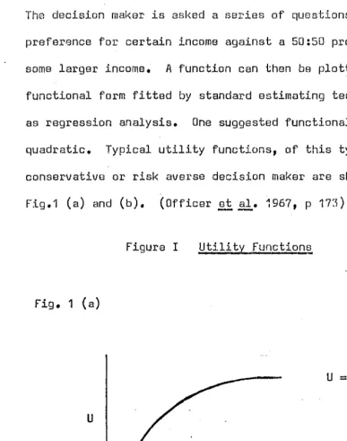
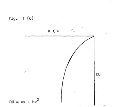
This method is based on the certainty-equivalent concept. The decision maker is asked a series of questions about his

preference for certain income against a 50:50 probability of

some larger income. A function can then be plotted and the functional form fitted by standard estimating techniques such as regression analysis. One suggested functional form is the quadratic. Typical utility functions, of this type, for a conservative or risk averse decision maker are shown in

Fig.1 (a) and (b). (Officer et ale

--

Figure I Utility Functions

Fig. 1 (a)

u

o x') 0

2

U

=

-Fig.. 1 (b)

x

<

-~---2

DU

=

ax

DU

Fig I (a) shows diminishing marginal utility for increasing 28 ..

returns and F1g I (b) shows increasing marginal dis.tJtili ty for increasing costs.

In practical terms the utility function can be expressed in terms of the expected value and variance of investment

projects where the function is assumed to be quadratic. This is represented by the first two moments of the probability distribution of the present value.

The quadratic utility function may be derived as follows.

,

'I·-~··'--··~---·'-· ..•••

t·~_~_.:c~:?::~-:-~-::~:;::~

r--__

.--,.o-.-~.-

given U ax + b 2 'x

..

then taking 8)(p8ctatiorls gj 1/8S ~,

E (u) _{"" E} (ax + bx2) e _"

then bocause Val' (x) - E(x 2· ) +

E (u) ₌₌ aE(x) -1- b Val' (x) +

where U

=

x == present value

a,b == constants

• • 0 ~ • 0

•

..

LE(x)]2 <J

• •

b[E(X)]2

_•

Equation (9) r8p~es8nts a ranking criterion expressed

in terms of the Expectation and variance of present value. This appears to be a major improvement over traditional methods) Unfortunately the concept of a utility function as

a proxy for the wellbei~g of society is reject~d by most

writers. r~ishan (1971, p 296) states lIit would seem quite

impractical to derive such a curve uniquely for ~ large number

of people; and f91' society .in general quite impossible." The expected present value of a project is not the gain

of a single person. It is th~ result of the aggregate gains

and losses of all people involve~ in the project. To replace

expected present value by total utility, the utilities of all

people aff~cted by the project have to be added together by

some arbitrary weighting system. This is clearly impossible.

Also, Arrow (1971, p 102) shows that use of quadratic functions

can lead to paradoxical results. The quadratiG function

30 ..

Dasgupta and Pearce (1972~ p 186) state that as yet

there is no generally accepted method for dealing with risk aversion in cost benefit analysis in a systematic waye They suggest that the only feasible alternative is to estimate the expected social utility and reduce it by a certain percentage depending on the extent of risk aversion thought to be

appropriate.

Little and Mirrlees (1974, p 319) suggest the USB of

the certainty equivalent approach where the deduction to be made from the expected present value on the account of

uncertainty should be the variance of the project divided by the gross national product of the country.

Another slightly different app:oach as sl.lggested by Fromm and Taubman (1968) is to present the policy making group with a series of assessments basad on a variety of utility functions, leaving the policy making group to make its own choice of utility function. Dillon (1971) reports that although this sounds far-fetched, similar procedures already operate in the Netherlands and some East European countries. There is one point that remains clear amid the murk of the risk aversion problem. This is that all projects should be evaluated in a systematic way at the risk-free rate of interest. If it is desired to take account of risk and

uncertainty it should be done in conjunction with the expected

present value calculated at that rate.

31.

2.,7 SU['W1Any

A case has been put for the evaluation of risk and uncertainty in agricultural projects, but on a review of evaluation techniques in use it has been found that many

deficiencies 8xist. In a search for a practical solution to the risk analysis problem we hav8 sesn that decision theory shows very little promise. The concept of utility as a

single meaSUre of the well-being of society, while being intrinsically neat, is impossible to derive at the national

level. Rather the solution is to make the risk and uncer-tainty explicit by presenting the present value in terms of its probability distribution - leaving it to the decision

maker to weight the expected outcome by its variance as he

sees fit. It should be the analyst's aim to present all the available and relevant information to the decision maker in an unbiased and explicit way. In the next two c .. hapters

32"

CHAPTGl 3

THE ANALYTICAL METHOD

This chapter outlines the steps involved in the

analytical method of evaluating risk and uncertainty in project appraisal. firstly it is shown how the mathematical

model was developed through the use of probability calculus. Then the following aspects of the model are discussed:

forecasting methods, the subjective probability distribution, correlation, and lastly the problems associated with the use of the model.

3.1 DEVELOPMENT Of THE MATHEMATICAL MODEL

Hillier (1963) laid the foundations of ris~ analysis.

His aim was to sho~ how, under certain circumstances, such

information as the probability distribution of the internal

rate of r8turn, present worth or annual cost of a proposed

investment could be derived. The approach used was similar

to that expounded by Merkowitz (1959) to determine the portfolio 1>.-.-:-.,

of mark~t shares to orovide the minimal variance of rate of _, .

return for a given expected rate of return. Hillier followed

Markowitz by u~ing the mathematics of combining random variables

to estimate the expected present value and variance of present

value of a projoct, given the mean and standard deviation for

The investment considered is one which would result" in cash flows over a number of years (where cash flows are

defined as money payments to or from a project).

Let X_t be the random variable that takes the value of

th

the net cash flow in the t year, where t

=

assume that X_{t has a normal distribu"i;ion with knolJJfl mean}

fir.

and st.andard deviation 0 t. Assume also that the relationships

betl~8en the X_{t for different t is either one of mutual}

independence or complete correlation. This forms a restrictive model which is rather unrealistic but it serves as a starting

point.

(a) Pr,obabiJ.l.ty Dist.!'..~bu.tion of the Pres.e,.nt Value.

The present value of the cash flow Ll year t (p t) is given by

=

• •

• •

•

where i equals the discount rate. It follows that the

expected present value is given by

:-n

E{P)

=

_~

t=o ••••••••• (11)

and if the X _0' X_1,

...

,

variance of the present value is given

by:-Val' (p)

_-

t

X

_....

_•

_•

_•

_{• •}

"t;=o _{( 1+i)2t}

where the Xo' X1 ••• , Xn are perfectly correlated the variance

becomes

34 ..

VEIl' (p) _'"=

t

[ n

" • • .. It G (13)

t:::.:o

In the case where ther8 are both i.n~8p8ndent flows (Yt )

and correlated flows (zk. Zk

0' 1 ' C 6 • t

the expected present value is

n E(Yt )

E(P) =

L

t=o • • • • 0 (14)

with varianceo

n

Var(Yt ) m ( n

car(z~r~~2

Val' (p)

_.

_~

_{I~'I t~o}

,\:::0 _(1+i)2t + _{(1+i) t}

In equations (14) and (15) it is assumed that the

z~

cash flows are perfectly correlated with the corresponding cash flows in other periods. For any given year, however, the cash flows are independent one with another.

Thus Hillier considers three

oases:-(i) independence between successive periods (ii) perfect correlation between periods

(iii) a net cash flow that is made up of an independent cash flow, plus m cash flows that are correlated between

periods (autocorrelated) but independent within a period.

(b) The Cen~~a~_Limit Theor~m. By reference to the

central limit theorem it can be concluded that the probability distribution_of the present value will be approximately normal

(Mood and Graybill, pp 149-153)~ This allows the use of the

normal tables to calculate the probability of obtaining any

35"

(c) ~nob.~f)8;~;:\~,ht~J?is.,t}'.tt~:0~igJJ_9.r !J3_R~ The Internal

Rate of Ret.urn (R) is defined as that value of i for which

P :::: 0" Ths projects accepted [n'8 those where R) i.

There is a certain amount of controversy regarding the acceptability of the IRR for general use in investment

appraisal (Hawkins and Poarce 1971 pp 29-38) but as the concern here is with methodology it will be assumed that the measure is acceptable.

The procedure for finding the probability distribution of the IRR is straightforward. An arbitrary value of i is selected and the probability distribution of P is calculated as described above. The next step is to find the probability

that P

<

<

Prob

~

<

=

t

<

1 ...

(16)

To find the cumUlative probability distribution of R,

the calculation of Prob

t

<

1

many values of i as desired.

Hillier

(1965)

(16)

" ••• should be viewed primarily as a computing e~uation for

practical application which is almost exact only when the IRR is a valid criterion IJJith probability essentially one."

Bernhard (1967) shows that the internal rate of return criterion is not valid in general. One of the major problems

is that of multiple real rootso de Faro

(1974)

36 ..

takes this problem into accounto Another problem ia that the

project's return is not independB~t of the cost of capital

and therefore the IRR criterion could give ambiguous and

incorrect results (Teichroew et

& ..

derived a FORTRAN program that takes this interdependence between project returns and the cost of capital into account.

Wagle (1967) extended Hillier's analysis by discussing methods to handle the cases where the means and variances of .the different cash flows were not known directly, but the means and variances of the factors which make up the cash flows aro known.

The net cash flow is derived from a number of distinct sources. Fer example, the net income from a project cuuld be a function of;-capital costs, operating costs, and revenue which may be derived from several soUrces. To allow for the relationships that occur between these sub cash flows they must be treated separately.

(a) lha Mean and Variance_cd' a Sum of Random Variables. Let the random variable Xtj denote the cash flow in period t

from the jth source where t=O,1,2, ••• , nand j=1,2, •••

,m.

It is assumed that Xtj has. a finite mean }ktj and variance

2

~tj. Then the net cash flow in period t is given by

37.

Thus the expected cash flow in period t is

m

:::

L

j==i

JJtj

, " ....

.

..

and the variance of the cash flow in period t is

m 2

2:

Var (X_{t )}

=

~

a

j=1 tj i

:;:j

It follows that the expected present value and variance of the present value are

n

E (p)

=

L

t=O where fA. == (11i) •• (20)

~,cov

(Xtj,XtJ)olt+tl

•• (21)

The covariances are functions of the correlation co-efficients and standard deviations between the variables. The covariance between different variables within the same period is

=

<S;i

This topic of correlation and dependency will not be elaborated here but left to a later section.