ISSN (Online): 2320-9364, ISSN (Print): 2320-9356
www.ijres.org Volume 4 Issue 7 ǁ July. 2016 ǁ PP. 01-11
Distribution Maps of TDS Concentration Using GIS At Assiut,
Egypt
Marco A. El-Dakar
1, A. Sefelnasr
2and M.M. Senosy
2 1Egyptian Environmental Affairs Agency, Assiut RBO2
Geology Department, Faculty of Science, Assiut University, Egypt
Abstract: The scarcity of water is one of the main issues in Egypt. In particular, the extreme climate in the form of less frequent rainfall affects the groundwater availability. Moreover, groundwater has been depleted by the increase in population. In this research, the spatial distribution of groundwatersalinity has been developed, and the prediction of groundwater total dissolved solid (TDS) has been made by using geostatistical analysis in geographic information system (GIS) software. The study area is the western flood plain from the River Nile in Assiut governorate located in the Upper Egypt. Ordinary kriging method was applied to map the spatial distribution of the groundwater chemistry for period 22 month (2009-2010). In predicting the total dissolved solid (TDS) concentration of groundwater distribution maps show increasing toward the western part of the Nile valley closed to western plateau. The lowest value of the total dissolved solid (TDS) concentrations of wells wasin the areas close to the River Nile, where the TDS concentration was low than 200pmmaround the year 2009 except in January, October, November and December, while the highest value of TDSconcentrations was in the area closed to Western Plateau in December 2009 and January 2010 (1000ppm).
Keywords: Groundwater quality. GIS.Geostatistics.Ordinary kriging .Semivariogram . Spatial distribution. TDS concentration
I.
INTRODUCTION
In order to discuss the role that groundwater may play in the management of regional water resources, the both surface water and groundwater are present in relatively significant quantities in a region. Actually, surface water and groundwater are not necessarily independent water resources. Base flow in streams is nothing more than groundwater emerging at ground surface. In this way, rivers and lakes, in direct, continuous hydraulic contact with adjacent or underlying aquifers serve as boundaries to the flow domain in the latter. By controlling groundwater levels in the vicinity of a spring, its discharge is controlled, or even stopped completely. The above considerations apply not only to water quantity, but also to water quality defined, for example by some chemical species or microorganisms carried with the water. Polluted surface water may easily reach and pollute groundwater and vice versa (Bear and Cheng, 2010).
Both surface water and groundwater are susceptible to man-made pollution, which usually requires costly remediation and treatment operations for its removal. In certain formations, pollutants may travel large distances in an aquifer without being attenuated. As for mineral contents in general the groundwater is more liable to picking up minerals in solution, although the range of concentrations encountered is very large. The removal of such minerals is usually very expensive. When groundwater does get polluted, the restoration of quality and the removal of pollutants is a very slow, hence, lengthy and sometimes practically impossible. This is due to the very slow movement of groundwater, especially in layers of very fine material, imbedded in formations of higher permeability and to adsorption and ion exchange phenomena on the surface of the solid matrix. These phenomena are especially significant when fine grained materialsare present in an aquifer (Bear and Cheng, 2010).
The objectives of the present research are to investigate theapplication of various spatial models and data transformationto interpret the spatial distribution of the groundwater total dissolved solid (TDS)at the western flood plain from the River Nile in Assiut governorate located in the Upper Egypt. In this study, kriging techniques in the framework of GIS software (ArcGISGeostatistical Analyst) are used.
1.1.Description of the study area and data collection
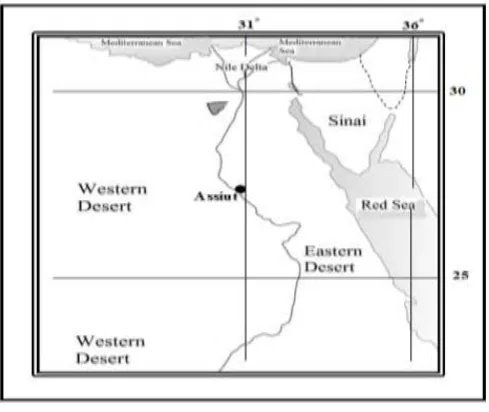
Assiut governorate is located on the River Nile at about 375 kilometers south of Cairo. It occupies a stretch of low land about 25926 square kilometers located between latitudes 27°8' and 27°40'North and longitudes 30°40' and 31°18' East (Figure 1). It is bordered from the east by the River Nile then a limestone Eocene plateau known locally as El-Gabal El-Sharki and from the west by another Eocene plateau known as El-Gabal El-Gharbi.
Figure 1: Location of Assiut Governorate.
The area under investigation as a part of Middle Egypt is characterized by semiarid to arid climatic conditions. It represents the central part of Upper Egypt and lies within the arid belt of North Africa. Its climate is hot, dry and almost rainless in summer, being mild with low rate of rainfall in winter.
All wells are utilized as the source of drinking water, in addition to agricultural and domestic uses. There are two types of water resources in Assiut governorate .These two resources are the Groundwater represented to the Quaternary aquifer and surface water represented to the River Nile with its irrigation system. The main irrigation canals have large length, width and depth. These canals are generally recharged directly from the River Nile at the upstream sides of the barrage which are constructed through the river course. Three main irrigation canals traverse the study area; Ibrahimiacanal, El Sohagiacanal and East Nag Hammadicanal. The precipitation is very low with 1.65 mm as the monthly average and temperature varies from 14 to 39 °C from winter to summer. Geologically, the study area lies between the Eocene limestone plateau from the west and the Recent Nile deposits from the east. It essentially a plain topography devoid of outcrops in most cases. The plain is covered by different Quaternary deposits (e.g. gravels, sands, silts, and clay). The elevation of the limestone plateau ranges from 80 to 180 m, whereas the elevation of the floor of the studied area varies from 35 to 90 m above sea level (Figure 2).
In the River Nile and canal, the total dissolved solid (TDS) concentration record 180 ppm while it reaches to300ppm in the Quaternary Aquifer. The difference in the concentrations of TDS may be due to many reasons such as ;(1) the exchange occur between surface water and groundwater outcome(surface water ground water interaction) which leads to reduce (TDS) concentration of wells near to surface water, by moving away from the surface water the concentrations will increase, (2) the population growth and activities led to high withdrawal amount of water from Quaternary Aquifer and this leads to increase the (TDS) concentration in the wells, (3) the rainfall have an important impact on the (TDS) concentration that means increase amount of rainfall lead to reduce the (TDS) concentration, (4) the lateral flux of water effects on the (TDS) concentrations, although all studies confirm that the Western Plateau is unkarstified limestone but in the actual there are many wells in the Western Plateau which gives sincerity to probability of impact of lateral flux of
water phenomenon on the (TDS) concentration. So it was important to study the occurrence and
distribution of (TDS) concentration in the Quaternary Aquifer.
II.
MATERIALS AND METHODS
Water samples were collected at selected wells to improve the understanding of the occurrence and distribution of concentrations of total dissolved solid (TDS) of the Quaternary Aquifer at the area under interest.1612water samples werecollected from 282 wells during the periodfrom January to December2009 (in Assiut city) except April 2009 (low recorded data) and the period from January to November2010 (inDayrout, Qusiya,Manfalout and Assiut city).
The water samples were collected after a minimum purge time of one minute at each well, ofcourse taking into account the predefined sampling standard methodology and precautions. Thesampling was conducted on monthlybasis; consequently, eleven sampling data datasets were obtained per year during the sampling period. The sampling database was improved and supported by the available data at the holding drinking water company for the same sampling period.
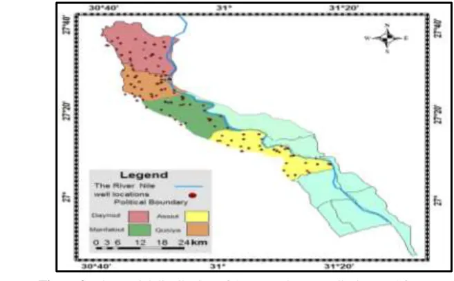
Figure (3) shows the spatial distribution of the wells from which the water samples were taken.
Figure 3: The spatial distribution of the groundwater wells that used for water sampling.
2.1 The Geostatisticsand Interpolation
2.1.1.Interpolation is a method of constructing new data points within the range of a discrete set of known data points. Interpolation is a procedure used to predict the values of cells at locations that lack sampled points. It is based on the principle of spatial autocorrelation or spatial dependence, which measures degree of relationship/dependence between near and distant objects (Childs, 2004).
2.1.2Geostatistics is a class of statistics used to analyze and predict the values associated with spatial or spatio-temporal phenomena. Geostatistics provides a means of exploring spatial data and generating continuous surfaces from selected sampled data points (ESRI, 2015). Geostatistics is intimately related to interpolation methods, but extends far beyond simple interpolation problems. Geostatistical techniques rely on statistical models that are based on random function (or random variable) theory to model the uncertainty associated with spatial estimation and simulation (Isaaks and Srivastava, 1989).
1989). Geostatistics goes beyond the interpolation problem by considering the studied phenomenon at unknown locations as a set of correlated random variables.
In geostatistical models, sampled data is interpreted as the result of a random process. The fact that these models incorporate uncertainty in their conceptualization doesn't mean that the phenomenon - the forest, the aquifer, the mineral deposit - has resulted from a random process, but rather it allows one to build a methodological basis for the spatial inference of quantities in unobserved locations, and to quantify the uncertainty associated with the estimator.
A value from locationχ1 (generic denomination of a set of geographic coordinates) is interpreted as a realizationz(χ1) of the random variableZ(χ1). In the spaceA, where the set of samples is dispersed, there areN realizations of the random variablesZ(χ1), Z(χ2),……., Z(χi), correlated between themselves.
The set of random variables constitutes a random function of which only one realization is knownz(χi) - the set of observed data. With only one realization of each random variable it's theoretically impossible to determine any statistical parameter of the individual variables or the function.
The proposed solution in the geostatistical formalism consists in assuming various degrees of stationarity in the random function, in order to make possible the inference of some statistic values. (Matheron, 1978).
For instance, if one assumes, based on the homogeneity of samples in areaA where the variable is distributed, the hypothesis that the first moment is stationary (i.e. all random variables have the same mean), then one is assuming that the mean can be estimated by the arithmetic mean of sampled values. Judging such a hypothesis as appropriate is equivalent to considering the sample values sufficiently homogeneous to validate that representation.
By applying a single spatial model on an entire domain, one makes the assumption that Z is a stationary process. It means that the same statistical properties are applicable on the entire domain. Several geostatistical methods provide ways of relaxing this stationarity assumption.
The hypothesis of stationarity related to the second moment is defined in the following way: the correlation between two random variables solely depends on the spatial distance between them, and is independent of their location: γ(Z(χ1), Z(χ2))= γ(Z(χ1), Z(χi+ h))2= γ(h)
Whereh=(χ1, χ2)=(χi, χi+ h)
This hypothesis allows measure the variogram based on the N samples: γ(h)=Σ(Z(χi) ـــZ(χi+ h))2
2.1.2. The variogram
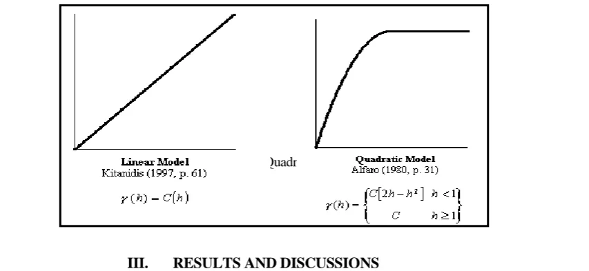
Surfer includes an extensive variogram modeling subsystem. This capability was added to Surfer as an integrated data analysis tool. The primary purpose of the variogram modeling subsystem is to assist you in selecting an appropriate variogram model when gridding with the kriging algorithm. There are several types of variogrammodel, this study was analyzed the data by two models (linear and Quadratic). The reason for using these models is the fixed equations of these models are match with the distribution of total dissolved solid concentration points (Figure 4) (Surfer tutorial).
Figure 4:The linear and Quadratic variogram models.
III.
RESULTS AND DISCUSSIONS
The spatial distribution of the chemical elements can give a good picture on the relationship between the surface water and the groundwater within the area under interest.
1
2
N
(h)
N (
h
)
3.1 The distribution of total Dissolved Solid (TDS) concentration in 2009
The amount of water flow ofthe main surface water such as theRiver Nile and the Ibrahimia canal was variable monthly during 2009 (Table 1), where it reaches to the minimum values in winter due to the winter embankment then it increase gradually to reach maximum values in summer months.
Table 1: The Water flow (Q) of Main surface water during 2009 in Assiut city.
Month The River Nile(Mm3) Ibrahimia canal(Mm3)
January 2124.06 297.6
February 2335.399 774.2
March 3197.948 952.6
April 3558.064 903.9
May 4199.009 921.9
June 4928.016 1090.7
July 5032.644 1160.8
August 4422.653 1135.6
September 2960.974 834.3
October 2869.559 764.8
November 2401.686 703.1
December 1866.772 555.1
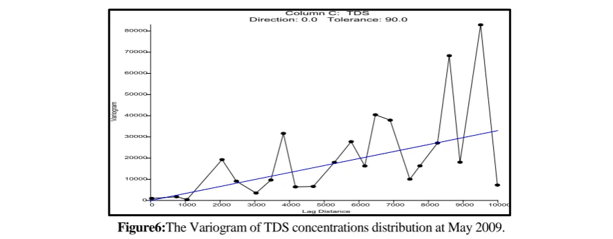
To assume the distribution and spatial variability of the Total Dissolved Solids within the area under interest, the values were handled by sophisticated geostatistical methods so as to apply the spatial distribution. The distribution of the Total Dissolved Solid (TDS) concentration ofwells in year 2009is located inAssiut city only (due to available data) except April 2009 due to low sampling records in this month. Figures(5, 6, 7 and 8) show the variogramsof TDSdistribution during year 2009represented byJanuary, May, August and December.
Using of surfer program show that the variogram of TDSdistribution of the January 2009 is linear with zero direction (90 tolerance and 1.6 slope) (Figure 5).The anisotropy is 3.1 ratios and 70 angles.
Figure5:The Variogram of TDS concentrations distribution at January 2009.
The variogram of TDSdistribution of the May 2009by using of surfer program is linear with zero direction (90 tolerances and 3.0 slopes) (Figure 6).The anisotropy is 1.1 ratios and 85 angles.
The variogram of TDSdistribution of the August 2009by using of surfer program is linear with zero direction (90 tolerances and 3.0 slopes) (Figure 7).The anisotropy is 1.3 ratios and 85 angles.
Figure7: The Variogram of TDS concentrations distribution at August 2009.
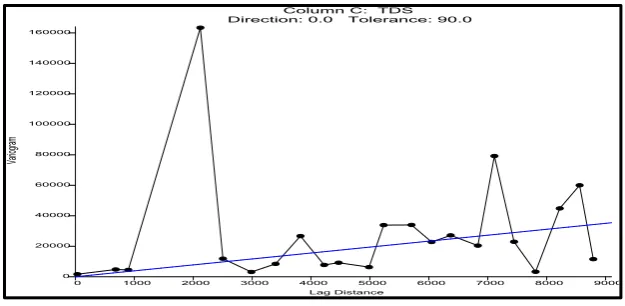
The variogram of TDSdistribution of the December 2009by using of surfer program is linear with zero direction (90 tolerances and 6.0 slopes) (Figure 8).The anisotropy is 1.2 ratios and 85 angles.
Figure8: The Variogram of TDS concentrations distribution at December 2009.
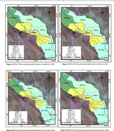
The Total Dissolved Solid (TDS) concentrations of wells are changing in areas and monthly during 2009. In the areas close to the River Nile, the TDS concentration range from 0.00ppm to 200pmm except in January, October, November and December reaches to 300 ppm. At the south part of valley, the TDS concentrations increase gradually from 200ppm at the area closed of the River Nile to reach 800ppm during December at western part of the valley. In the middle of valley where the Ibrahimia canalpresents, the majority of TDS concentrations were 300ppm and 400ppm while it reach to 500ppm in January and February. By reaching to Western Plateau, the TDS concentrations ranging between 700ppm to 900ppm, the minimum value is 600ppm in July and records the maximum value (1000ppm) in December (Figures 9 to 19).
3.2 The distribution of total Dissolved Solid (TDS) concentration in 2010
The amount of water flow ofthe main surface water such as theRiver Nile and the Ibrahimia canal was variable monthly during 2010 (Table 2), where it reaches to the minimum values in winter due to the winter embankment then it increase gradually to reach maximum values in summer months.
Table 2: The Water flow (Q) of Main surface water during 2010 in Assiut.
Month The River Nile(Mm3) Ibrahimia canal(Mm3)
January 1858.204 324.88
February 2238.282 677.6
March 2815.58 847.1
April 2950.622 805.4
May 3804.126 868.5
June 4765.755 1043.3
July 4856.73 1114.3
August 4380.476 1132.5
September 2902.207 845.3
October 2936.411 794.5
November 2478.635 713.6
December 1770.498 552.7
Using of surfer program show that the variogram of TDSdistribution of the January 2010is Quadratic with zero direction, 90 tolerances, 62800scales and 14500 lengths (Figure 20).The anisotropy is 2.5ratios and 115angles.
Figure20:The Variogram of TDS concentrations distribution at January 2010.
The variogram of TDSdistribution of the June 2010by using of surfer program is Quadratic with zero direction, 90 tolerances, 26800 scales and 17900 lengths (Figure 21) .The anisotropy is 1.45 ratios and 90 angles.
Figure21:The Variogram of TDS concentrations distribution at June 2010.
REFFERENCES
[1]. Ayazi, M. H.; Pirasteh, S.; Arvin, A. K. P.; Pradhan, B.; Nikouravan, B. and Mansor, S. (2010): Disasters and risk reduction in groundwater: Zagros Mountain Southwest Iran using geoinformatics techniques. Disaster Adv 3(1):51–57.
[2]. Bear, J. and Cheng, A. H. (2010): Modeling Groundwater Flow and Contaminant Transport. Springer Science, Business Media B.V., 834pp. [3]. Childs, C. (2004): Interpolating Surfaces in ArcGIS Spatial Analyst. ESRI Education Service, Redlands.
[4]. El Afly, M. (2012): Integrated geostatistics and GIS techniques for assessing groundwater contamination in Al Arish area, Sinai, Egypt. Arab J Geosci 5(2):197–215. doi:10.1007/s12517-010- 0153-y.
[5]. ESRI (Environmental Systems Research Institute) (2015): Arc Map 10.x. ESRI Press, Red lands, California.
[6]. Isaaks, E. H. and Srivastava, R. M. (1989): An Introduction to Applied Geostatistics. Oxford University Press, New York, USA. [7]. Kumar, V. and Remadevi (2006):Kriging of groundwater levels—a case study. J Spat Hydrol 6(1):81–92.
[8]. Machiwal, D.; Mishra, A.; Jha, M. K.; Sharma, A. and Sisodia, S. S. (2012): Modeling short-term spatial and temporal variability of groundwater level using geostatistics and GIS. Arab J Geosci 21(1):117–136. doi:10. 1007/s11053-011-9167-8.
[9]. Manap, M.A.; Nampak, H.; Pradhan, B.; Lee, S.; Sulaiman, W. N. A. and Ramli, M. F. (2012): Application of probabilistic-based frequency ratio model in groundwater potential mapping using remote sensing data and GIS. Arab J Geosci.doi:10.1007/s12517-012-0795-z. [10]. Mehrjardi, R. T.; Jahromi, M. Z.; Mahmodi, S. and Heidari, A. (2008): Spatial distribution of groundwater quality with geostatistics (case
study: Yazd-Ardakan Plain). World ApplSci J 4(1):9–17.
[11]. Neshat, A.; Pradhan, B.; Pirasteh, S. and Shafri, H. Z. M. (2013): Estimating groundwater vulnerability to pollution using modified DRASTIC model in the Kerman agricultural area. Iran Environ Earth Sci. doi: 10.1007/s12665-013-2690-7.