www.ijres.org Volume 4 Issue 11 ǁ
November. 2016 ǁ
PP.50-55
Frequency Analysis of aFree Vibrating SSCC Thin Rectangular
Orthotropic Plate Using Improved Rayleigh’s Method.
D.O Onwuka
1, O.M Ibearugbulem
2, A.C Abamara
3, C.F Njoku
4, S.I Agbo
51,2,4,5(Department Of Civil Engineering, Federal University Of Technology, Oweeri) 3
(Federal Ministry Of Transport, Abuja, Nigeria)
Abstract:
This paper presents the solution of the analysis of free vibration of a rectangular thin orthotropic plate using an improved Rayleigh’s method. The plate is bounded by two adjacent simply supported edges (i.e. SS) and another two adjacent clamped edges (i.e. CC). The total potential energy functional of a free vibrating plate, was derived from first principle, using the theory of elasticity. A truncated Taylor’s Mclaurin series of fourth terms was used to develop a general deflection function that satisfies the boundary conditions of the given plate. The deflection function was then, substituted into the potential energy functional and the resulting equation subsequently minimized. Thereafter, the equation for natural frequency, λ, of the SSCC plate was determined, and used to obtain natural frequencies for aspect ratios ranging from 0.1 to 2.0, in steps of 0.1. These average percentage differences, indicate that the formulated deflection function for the clamped plate, is a very good approximation to the exact deflection function of the free vibration of a clamped rectangular thin orthotropic plate.Keywords:
Clamped Rectangular Plate, Free Vibration Analysis, Improved Rayleigh’s Method, Natural Frequency, Orthotropic Vibrating Plate, and Shape Function.I.
INTRODUCTION
[1] Obtained the exact solution of large deflections analysis of clamped circular plates. [2]Used Ritz method in the analysis of plated with opposite sides simply supported and other possible combinations of clamped, simply supported and free edge conditions and presented their analytical results. [3], conducted the free vibration analysis of isotropic and anisotropic rectangular thin plates subjected to general boundary conditions using a modified Ritz method. [4] Applied the method of superposition to the vibration analysis of rectangular plates with a combination of clamped and simply supported boundary conditions. [5], using novel separation of variables, obtained the exact solutions for free vibrations of rectangular thin orthotropic plates with all combinations of simply supported and clamped boundary conditions. One of the plate cases he considered is the SSCC plate. [6], using Taylor’s series function in Rayleigh-Ritz method, obtained a new approximate solution of SSCC plate.
II.
THEORITICAL
FORMULATION
2.1 Differential Equation of a Thin Rectangular Orthotropic Plate in Vibration.
[5] Derived the following governing differential equation of a thin orthotropic plate experiencing free vibration:
D1
∂4w(x, y, t)
∂x4 + 2D3
∂4w(x, y, t)
∂x2dy2 + D2
∂4w(x, y, t)
∂y4 ρh
∂2w
∂t2 x, y, t = 0 (1)
WhereD1, D2 and D3 are flexural rigidities of the plateW x, y, t is the deflection function of the plate
x and y are cartesian co-ordinate of the plate. t = thickness of the plate.
ρ = density of the material h = plate thickness
Using Taylor –Maclaurin series, [7] expressed the shape function, w as follows:
W = W x, y = F
m x
0 F n y0
m! n! (x − x0)
m. (y − y 0)n (2)
∞
n=0
∞
m =0
WhereF m x
0 is the mth partial derivative of the function, w, with respect to x.F n y0 is the nth
partial derivative of the function, w, with respect to y, m! and n! are the factorials of m and n respectivelyx0 and
y0 are the points of origin.
W = ImJn xm. yn (3) 4
n=0 1
m=0
Expressing Equation (3) in terms of non-dimensional co-ordinates, R and Q, yields Equation (4)
w = ambn RmQn (4)
4
n=0 4
m =0
where
am= Im. am (5)
and
bn = Jn. bn(6)
But R = x/a and Q = y/b (7)
The function given by Equation (4) can be further expanded in the following form:
w R, Q = a0+ a1R + a2R2+ a3R3+ a4R4 b0+ b1Q + b2Q2+ b3Q3+ b4Q4 (8)
Whereai and bi (i= 0,1,2,3,4) are constants.
2.2 Boundary Conditions of SSCC Orthotropic Plate.
The thin rectangular orthotropic plate considered in this work, has two adjacent simply supported edges and another two adjacent clamped edges as shown in Fig 1.
The edges AD and DC are simply supported, while edges AB and BC are clamped.
For simply supported edges, the deflections and bending moment vanishes. The boundary conditions for the SSCC plate, are as follows:
W R = 0 = 0 ; W′R R = 0 = 0
W R = 1 = 0 ; W′R R = 1 = 0
W Q = 0 = 0 ; W′Q Q = 0 = 0
W Q = 1 = 0 ; W′′Q Q = 1 = 0
Substituting successively, the boundary conditions, W 𝐑 = 𝟎 = 𝟎 ,𝐖′𝐑 𝐑 = 𝟎 = 𝟎, 𝐖 𝐐 = 𝟎 = 𝟎, and
𝐖′𝐐 𝐐 = 𝟎 = 𝟎 into the Equation (8) yields:
𝑎0= 0 (9)
𝑎1= 0 (10)
𝑏0= 0 (11)
𝑏1= 0 (12)
Similarly, substituting successively, the boundary conditions, 𝐖 𝐐 = 𝟏 = 𝟎 and 𝐖′′𝐐 𝐐 = 𝟏 = 𝟎 into Equation (8), gives respectively:
𝑎2+ 𝑎3+ 𝑎4= 0 (13)
2𝑎2+ 6𝑎3+ 12𝑎4= 0 (14)
Solving Equations (13) and (14), yields the following:
𝑎1= 1.5𝑎4and𝑎3 =2.5 𝑏4 (15)
Substituting these values of a1, and a2, into Equation (8), gives the following displacement function, W.
W =𝑎4𝑏4(1.5𝑅2− 2.5𝑅3+ 𝑅4)(1.5𝑄2− 2.5𝑄3+ 𝑄4) (16)
where:
A is the amplitude of the deflected shape=𝑎4𝑏4 (18)
H is the deflected shape = (1.5𝑅2− 2.5𝑅3+ 𝑅4)(1.5𝑄2− 2.5𝑄3+ 𝑄4) (19)
2.3 Application of Variational Principle.
The differentiation of the partial derivatives of the deflected shape, H, with respect to the dimensionless parameters, R and Q, are as follows:
W′R = A∂H
∂R (20)
W′′R = A∂2H
∂R2 (21)
W′Q= A∂H
∂Q (22)
W′′Q = H∂2H
∂Q2 (23)
W′′RQ = A ∂2H
∂R ∂Q (24)
Squaring and integrating partially the Equations (17), (21),(23) and (24) with respect to R and Q in close domain, yields equations (25),(26),(27) and (28) respectively.
(AH)01 01 2∂R ∂Q = 0.0000056846813A2 (25)
(A∂2H
∂R2)
2∂R ∂Q =
1 0 1
0 0.013572A
2 (26)
(A∂2H
∂Q2)
2∂R ∂Q =
1 0 1
0 0.013572A
2 (27)
(A ∂2H
∂R ∂Q) 2 1
0 1
0 ∂R ∂Q = 0.0073469A
2 (28)
III.FORMULATION
OF
NATURAL
FREQUENCY
EQUATION
FOR
A
VIBRATING
THIN
RECTANGULAR
ORTHOTROPIC
PLATE.
The total potential energy functional, Π, is given by Equation (29)
U = Π – KE (29)
where U = strain energy KE = Kinetic Energy. But, U = Dx
2b2 [ φ1 p3 1 0 1 0 (H
∂2H ∂R2)
2 + 2 φ2
p (H
∂2H ∂R ∂Q)
2+pφ 3(H
∂2H ∂Q2)
2]∂R ∂Q (30)
And, the kinetic energy, KE, is given as: K.E= pb2λ
2ρt
2 (AH)
2 1 0 1
0 ∂R ∂Q (31)
where P = aspect ratio λ = natural frequency
Substituting the value of strain energy U and kinetic energy, KE into Equation (29) gives Equation (32):
Π= Dx
2b2 [
φ1 p3 1 0 1 0 (H
∂2H ∂R2)
2+2φ2
p (H
∂2H ∂R ∂Q)
2+pφ 3(H
∂2H ∂Q2)
2]∂R ∂Q −pb2λ2ρt
2 (AH)
2 1 0 1
0 ∂R ∂Q (32)
where φ1= Dx
Dx = 1 (33)
φ2 = B
Dx (34)
and φ3 = Dy
Dx (35)
Minimizing the Equation (32) yields: ∂Π
∂A= DxA
b2 [
φ1 p3 1 0 1 0 (∂ 2H
∂R2) 2+ 2φ2
p (
∂2H
∂R ∂Q)
2+ pφ 3(
∂2H
∂Q2)
2] ∂R ∂Q − pAb2λ2ρt H 2 1
0 1
0
∂R ∂Q (36)
Rearranging the Equation (36), gives natural frequency squared,λ2
λ2= Dx
b4ρt [ φ1
p4
∂2H ∂R2
2
+2φ2
p2
1 0
∂2H ∂R ∂Q
2
+φ3 ∂2H
∂Q2
2
∂R ∂Q
1 0
H1 2∂R ∂Q 0
1 0
(37)
(ii) λ2 in terms of a and b, gives Equation (38)
λ2
=
Dx
a4ρt [φ1 ∂2H ∂R2
2
+ 2φ2a2 1
0
∂2H ∂R ∂Q
2
+φ3a4 ∂2H ∂Q2
2
∂R ∂Q
1 0
b2 (38)
(iii) λ2 in terms of a and b, yields Equation (39)
λ2= Dx
a4ρt [φ1
∂2H
∂R2 2
+ 2φ2a2 1
0
∂2H
∂R ∂Q
2
+φ3a4 ∂ 2H ∂Q2 2 ∂R ∂Q 1 0 (39)
(b) For aspect ratio,p = b a , the square of the natural frequency, λ2, is given by Equation 40 .
(i)𝜆2𝑖𝑛𝑡𝑒𝑟𝑚𝑠𝑜𝑓𝑝𝑎𝑛𝑑𝑏𝑔𝑖𝑣𝑒𝑠𝑒𝑞𝑢𝑎𝑡𝑖𝑜𝑛 40
λ2
=
Dx
a4ρt [φ1 ∂2H ∂R2
2
+2φ2
p2
1 0
∂2H ∂R ∂Q
2
+φ3
p4
∂2H ∂Q2
2
∂R ∂Q
1 0
H1 2∂R ∂Q 0
1 0
(40)
Substituting the relevant Equations (25) – (28) into the Equation (37) and simplifying the resulting Equation yields Equation (41)
λ2= Dx
b4ρt
φ1
p4∗ 238.746 +
φ2
p3∗ 258.481 +φ3∗ 238.746 ; for p =
a
b 41
In terms of a and p, the Equation 41 becomes Equation (42)
λ2
= Dx
a4ρt φ1∗ 238.746 +φ2∗ 258.481p
2+φ
3∗ 238.746p
4 ; for p =a
b 42
In terms of ‘a’ and ‘b’, Equation (41) represented as Equation (43)
λ2= Dx
a4ρt φ1∗ 238.746 +
φ2∗ a2
b2 ∗ 258.481 +
φ3a4
b4 ∗ 238.746 ; for p =
a
b(43)
Then, for the reciprocal of the aspect ratio (i.e) p=b a , the square of the fundamental frequency is given by equation (44)
λ2= Dx
a4ℯt φ1∗ 238.746 +
φ4
p2∗ 258.481 + φ3
p4∗ 238.746 ; for p=b a (44) where φ1=Dx
Dx
,φ2= B Dx
,φ3=Dy Dx
The fundamental frequencies, λi , are the roots of Equations (41)-(44). These fundamental frequencies, λ, of an
SSCC plate, can be obtained for various value ofaspect rations, p=b a and combinations of flexural rigidities,φ1,φ2 and φ3.
However, the exact solution can be obtained from the following expression given by Xing and Liu (2009). 𝐷1
𝜕4𝑤
𝜕𝑥4 + 2𝐷3
𝜕4𝑤
𝜕𝑥2𝜕𝑦2+ 𝐷2
𝜕4𝑤
𝜕𝑦4 − 𝛽
4𝑤 = 0
IV.
RESULTS
AND
DISCUSSION
The Equations (42) and (44), were used to determine the fundamental frequencies,λ , for various aspect ratios, p=b a and different combinations of flexural rigidities, φ1, φ2 and φ3 of an SSCC thin rectangular orthotropic plate undergoing free vibration. The results obtained are presented in Tables 1-3. Also the solution by [5] and[8], for aspect ratios, (p=b a) of 0.5, 1.0 and 2.0, are given in the same Tables 1-3.
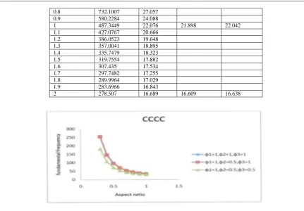
Besides, the graph of fundamental frequencies,λ , and aspect ratios, p=b a, (given in Tables 1-3), are plotted for various combinations of flexural rigidities φ1 φ 2 and φ3 (see Fig 2). The diagram shows that there is high convergence of the three curves as the aspect ratio increased.
Table 1: Fundamental frequencies, λ ,of a free vibrating SSCC plate for various aspect ratios, p=b a, and flexural rigidities, φ 1= φ 2= φ 3= 1
Aspect Ratios, p=ba,
New solution Exact solution,
λ2
Kantorovich’s Solution, λ3
λ12 λ1
0.1 2413451 1553.528
0.2 155911 394.856
0.3 32584.37 180.511
0.4 11179.88 105.735
0.5 5092.441 71.361 70.877 71.081
0.6 2798.84 52.904
0.7 1760.569 41.959
0.8 1225.465 35.007
0.9 921.7203 30.360
1 735.9535 27.128 26.867 27.059
1.1 615.417 24.808
1.2 533.3682 23.095
1.3 475.2718 21.801
1.4 432.7593 20.803
1.5 400.7745 20.019
1.6 376.1337 19.394
1.7 356.7601 18.888
1.8 341.2564 18.473
1.9 328.6568 18.129
2 318.2776 17.840 17.719 17.770
where λ= fundamental frequency , λ2= fundamental frequency squared.
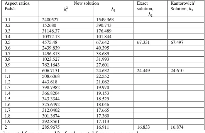
Table 2: Fundamental frequencies, λ, of a free vibrating SSCC plate for various aspect ratios, p=b a and flexural rigidities, φ =φ3=1 and φ2=0.5
Aspect ratios, P=b/a
New solution Exact
solution,
λ2
Kantorovich’ Solution, λ3
λ12 λ1
0.1 2400527 1549.363
0.2 152680 390.743
0.3 31148.37 176.489
0.4 10372.13 101.844
0.5 4575.48 67.642 67.331 67.497
0.6 2439.839 49.395
0.7 1496.813 38.689
0.8 1023.527 31.993
0.9 762.1643 27.601
1 606.7131 24.632 24.449 24.610
1.1 508.6068 22.552
1.2 443.618 21.062
1.3 398.7982 19.970
1.4 366.8204 19.153
1.5 343.3344 18.529
1.6 325.6492 18.046
1.7 312.0402 17.665
1.8 301.3674 17.360
1.9 292.8561 17.113
2 285.9675 16.911 16.833 16.874
where λ= fundamental frequency , λ2= fundamental frequency squared.
Table 3: Fundamental frequencies, λ, of a free vibrating SSCC plate for various aspect ratios, p=b a and flexural rigidities, φ =1, φ3=0.5 and φ2=0.5.
Aspect Ratios, p=ba,
New solution Exact solution,
λ2
Kantorovich’s Solution, λ3
λ12 λ1
0.1 1206845 1098.565
0.2 78074.87 279.419
0.3 16411.55 128.108
0.4 5709.309 75.560
0.5 2665.589 51.629 51.302 51.507
0.6 1518.788 38.972
0.8 732.1007 27.057
0.9 580.2284 24.088
1 487.3449 22.076 21.898 22.042
1.1 427.0767 20.666
1.2 386.0523 19.648
1.3 357.0041 18.895
1.4 335.7479 18.323
1.5 319.7554 17.882
1.6 307.435 17.534
1.7 297.7482 17.255
1.8 289.9964 17.029
1.9 283.6966 16.843
2 278.507 16.689 16.609 16.638
Fig 2: Graph of fundamental frequency, λ against aspect ratio, p
V.
CONCLUSION
The closeness of the fundamental frequencies, λ, from the three methods, underscores the similarity in the deflection functions chosen in the three methods. The new equations formulated in this work, can be used to compute very close approximation of the fundamental frequencies of an SSCC thin rectangular orthotropic plate undergoing vibration. And the newly formulated equations, give upper bound values of the fundamental frequencies.
The convergence of the three curves given in Fig 2, indicates that the fundamental frequency at a certain value of the aspect ratio (i.e. at about p=b a= 1), becomes approximately constant, irrespective of the combination of the flexural rigidities, φ 1 ,φ 2 and φ 3.
And, the use of Taylor’s series in Rayleigh- Ritz method, overcomes the limitations encountered in the derivation of fundamental frequency using conventional methods.
REFERENCES
[1]. S. Way, Bending of circular plates with deflection, ASME J.Appl. Mech., 56, 1934pp. 627-636. [2]. A.W.Leissa,The free vibration of rectangular plates, J. Sound Vib.1973, 31, pp 257-293.
[3]. Y. Narita, Combinations for the Free-Vibration Behaviors of Anisotropic Rectangular Plates under General Edge Conditions. ASME J.Appl.Mech., 67, 2000,pp.568-573.
[4]. D.J. Gorman, Free Vibration 0f Cantilever Plates by method of Super-Position, J . Sound Vib.,1976. pp 453 – 467.
[5]. Y. F. Xing, and B. Liu, New Exact Solutions for Free Vibrations of Thin Orthotropic Rectangular Plates. The Solid Mechanics Research Center, Beijing University of Aeronautics and Astronautics, Beijing 100083, China. Composite Structures Journal Homepage: Available at www.elsevier.com/locate/compstruct. (2009).
[6]. A. C.Abamara, Free Vibration Analysis of Material Orthotropic Rectangular Thin Plates Using Taylor-Maclaurin Series In Rayleigh Ritz Method. M.Sc Research work Submitted to the Department of Civil Engineering Federal University Of Technology Owerri, Nigeria, 2014.
[7]. O. M. Ibearugbulam, Application of a Direct Variational Principle in Elastic Stability Analysis of Thin Rectangular Isotropic Plates. Ph. D Thesis Submitted To Federal University of Technology, Owerri, Nigeria, 2012.