A Hypercube-based Scalable Interconnection
Network for Massively Parallel Computing
LIU Youyao
Microelectronics School, XIDIAN University, Xi’an, 710071, China [email protected]
HAN Jungang and DU Huimin
Xi'an Institute of Posts & Telecommunications, Xi’an, 710121, China {hjg, fv}@xiyou.edu.cn
Abstract - An important issues in the design of interconnection networks for massively parallel computers is scalability. A new scalable interconnection network topology, called Double-Loop Hypercube (DLH), is proposed. The DLH network combines the positive features of the hypercube topology, such as small diameter, high connectivity, symmetry and simple routing, and the scalability and constant node degree of a new double-loop topology. The DLH network can maintain a constant node degree regardless of the increase in the network size. The nodes of the DLH network adopt the hybrid coding combining Johnson code and Gray code. The hybrid coding scheme can make routing algorithms simple and efficient. Both unicasting and broadcasting routing algorithms are designed for the DLH network, and it is based on the hybrid coding scheme. A detailed analysis shows that the DLH network is a better interconnection network in the properties of topology and the performance of communication. Moreover, it also adopts a three- dimensional optical design methodology based on free-space optics. The optical implementation has totally space- invariant connection patterns at every node, which enables the DLH to be highly amenable to optical implementation using simple and efficient large space-bandwidth product space-invariant optical elements.
Index Terms - interconnection network, scalability, massively parallel computing, hypercube, double-loop, optical interconnect
I. INTRODUCTION
Advances in hardware technology, especially the VLSI circuit technology, have made it possible to build a large-scale multiprocessor system that contains thousands or even tens of thousands of processors [1]. For example, the Connection Machine contains as many as 216 processors [2]. One crucial step on designing such a multiprocessors system is to determine the topology of the interconnection network (network for short), because the system performance is significantly affected by the network topology. The binary n-cube, also called
hypercube, network has been proved to be a very powerful topology [3,4,5]. The attractiveness of the hypercube topology is its small diameter, which is the
maximum number of links (or hops) a message has to travel to reach its final destination between any two nodes. For a hypercube network the diameter is identical to the degree of a node n= log2N. There are 2n nodes contained in the hypercube; each is uniquely represented by a binary sequence bn−1bn−2...b0 of length n. Two nodes in the hypercube are adjacent if and only if they differ at exactly one bit position. This property greatly facilitates the routing of messages through the network. In addition, the regular and symmetric nature of the network provides fault tolerance [6].
Among important parameters of an interconnection network of a multicomputer system are its scalability and modularity [6,7]. Scalable networks have the property that the size of the system (e.g., the number of nodes) can be increased with minor or no change in the existing configuration. Also, the increase in system size is expected to result in an increase in performance to the extent of the increase in size.
hypercube. Since the topology of HHC is closely related to the topology of the hypercube, HHC inherits some favorable properties from the hypercube. Nevertheless, HHC still suffers from the limitation of scalability because of not be constant node degree.
Existing research has proposed some networks that are variations of the hypercube. These variants include the Exchanged Hypercube [5], the Gaussian Hypercube [10], and the Reduced Hypercube [11]. They are defined by removal of a portion of the n-cube’s links while
attempting to minimize performance degradation. Reduction of link complexity invariably makes the network more cost effective as it scales up. Nevertheless, some usefulness of a richer connectivity disappears. Routing becomes a serious problem, particularly when faulty components exist. Most hypercube-based interconnection networks are proposed in the literatures [12,13,14,15,16] suffer from similar size scalability problems. The Optical Multi-Mesh Hypercube (OMMH) [6] is a network that combines the positive features of the hypercube with those of a mesh. The OMMH can be viewed as a two-level system: a local connection level representing a set of hypercube modules and a global connection level representing the mesh network connecting the hypercube modules. The Spanning Multi-channel Linked Hypercube (SMLH)[7] possesses a constant degree and a constant diameter while preserving many properties of the hypercube. Nevertheless, the Routing of two scalable network becomes more complex than the hypercube.
A new scalable network topology, called Double-Loop Hypercube (DLH(m,d)), is proposed in this paper, which
combines advantages of both the hypercube topology, such as small diameter, high connectivity, symmetry and simple routing, and the scalability and constant node degree of a new DL(2m) topology. The nodes of the
DLH(m,d) network adopt the hybrid coding combining
Johnson code and Gray code. Two nodes in the DLH(m,d)
are adjacent if and only if they differ at exactly one bit position. The hybrid coding scheme can make routing algorithms simple and efficient. The DLH(m,d) network
can maintain a constant node degree regardless of the increase in the network size. It is proved that the DLH(m,d) is of characteristics such as regularity and
good scalability.
Optics, owing to its inherent parallelism, high spectral and spatial bandwidth, and low signal cross talk, possesses the potential for a better solution to the communication problem in parallel and distributed computing [6,7,17,18]. Some studies have shown that free-space optical interconnects provide far better communication bandwidth and power dissipation for sufficiently long connection paths that is possible with VLSI technology [19,20]. A totally space-invariant system has a very regular structure where all the nodes have the same connection patterns which consequently lower the design complexity. There is a fundamental trade-off between the space-bandwidth product, the total degree of freedom in an optical interconnect (the space is considered the cross section area and the bandwidth is the
highest spatial frequency handled by the system), and the degree of space-variance. A totally space-invariant system has minimal space-bandwidth product requirements, whereas a totally space-variant system has extensive space-bandwidth product requirements. Also, totally space-invariant systems are much easier to implement than totally space-variant systems[6,7,17,18].
Therefore, we have adopted a three-dimensional (3-D) optical implementation for the DLH(m,d). The
implementation methodology was proposed by Ahmed Louri [6,7,17,18]. The distinctive advantages of the implementation methodology include: i) an efficient and scalable interconnection network, ii) better utilization of the space-bandwidth product ofoptical imaging systems, iii)full exploitation of the parallelism of free-space optics, iv)simple optical implementations because of the use of large space-bandwidth product space-invariant optical elements, v) cost-efficient implementations because the beams which will be directed orthogonal to the device plane would share the same set of imaging optics for interconnects, and consequently, the cost of the optical hardware would be shared by a large amount of communicating elements, and vi) compatibility with the two-dimensional (2-D) optical logic and switching, and optoelectronic integrated circuit technologies [6].
The rest of the paper is organized as follows. Section II discusses the topology architecture ofDLH(m,d). Routing
algorithms and the properties of the DLH(m,d) are
discussed in section III and section IV. In section V, optical implementation issues, including 3-dimensional construction, of the DLH(m,d) are addressed. Section 6
concludes the paper.
II. DLH(m,d) INTERCONNECTION NETWORK
A. Preliminaries
Definition 1. Binary unit-distance cyclic code is a
binary code whose each two adjacent codes have one and only one bit different(unit distance characteristic), and the first code and the last one in those codes have one and only one bit different(cycle characteristic).
Definition 2. Binary code represents each number in
the descending sequence of integers {n-1,n-2,…,2, 1,0}
as a binary string of length m=
⎡
n
/
2
⎤
by an order. The binary code has the properties of definition 1 and as follows: i) for 0<k<m, Q=Zm-1…ZkOk-1…O0(Zi stands for0, Ojstands for 1, k≤i≤m-1,0≤j≤k-1) is the code of integer
k; ii) for k>m, Q=Om-1…Ok-mZk-m-1…Z0(Zi stands for 0,
Oj stands for 1, 0≤i≤k-m-1,k-m≤j≤m-1) is the code of
integer k; iii) for k
≡
m, Q=Om-1…O0(Oi stands for 1,0≤i≤m-1) is the code of integer k; iv) for k
≡
0, Q=Zm-1…Z0(Zi stands for 0, 0≤i≤m-1) is the code ofinteger k. This binary code is called Johnson code. Definition 3. Double-Loop (DL(2m)) interconnection
network is a kind of network topology with the following characteristics: i) The DL(2m) has 4m nodes and 6m links,
which consists of two rings, an outer ring and an inner ring, each containing 2m nodes; ii) The nodes of the
outer/inner ring of the DL(2m) can be marked with m bits
where the outer ring is marked sign 1 and the inner ring is 0; iii) In which the coding rules of the nodes are as follow: When there is just one bit different between any two nodes, there will exist a link between them, that is to say, these two nodes are neighboring to each other.
An example of a DL(2m) is shown in figure 1, where m
equals to 4, which is composed of 4×4=16 nodes and 6
×4=24 links. The nodes of the outer/inner ring of the DL(2m) can be marked with 4 bits Johnson code and 1 bit
ring sign at most significant bit, where the outer ring is marked sign 1 and the inner ring is 0. The topology of the DL(2m) is simple, symmetric and scalable in architecture,
and it is 3-regular plane graph.
u7=11000
u6=11100
u5=11110 u4=11111
u3=10111 u2=10011
u1=10001 u0=10000
v7=01000 v6=01100
v5=01110 v4=01111 v3=00111 v2=00011
v1=00001 v0=00000
Figure 1. DL(2m) network, where m equals to 4.
Definition 4. n dimensional Hypercube Interconnec-
tion Network(n-cube) is a kind of network topology with
the following characteristics: 1) which is composed of 2n
nodes and n*2n-1 links; 2) in which any node can be
coded with a different binary string of n bits such as bn−1bn−2...b0; 3) In which the coding rules of the nodes are as follow: When there is just one bit different between any two nodes, there will exist a link between them, that is to say, these two nodes are neighboring to each other.
Figure 2 illustrates the topology of the 4 dimensional hypercube networks, which is composed of 24=16 nodes and 4·24-1=32 links, and in which the nodes are coded from 0000 to 1111.
B. Topology of the DLH(m,d) Network
The total number of nodes in the DLH(m,d) is 4m×2d.
When m≥2, the DLH(m,d) can be constructed by
combining the positive features of the hypercube topology, such as small diameter, high connectivity, symmetry and simple routing, and the scalability and constant node degree of the DL(2m) topology as follows:
1) The 2dnodes can be connected to be a
d dimensional
hypercube network according to definition 4, in which any node can be coded with a node-id, which adopts Gray
codefrom 0 to d. So, we will obtain 4m such kinds of d
dimensional hypercube networks.
2) The 4m such kinds of d dimensional hypercube
networks can be divided into 2m groups, in which any
group can be coded with a group-id, which adopts Johnson code from 0 to 2m, and any d dimensional
hypercube network in a same group can also be coded with a net-id using 0 or 1.
3) The nodes with both the same node-id in different groups can be connected to a DL(2m) according to
definition 3.
4) The code of nodes in the DLH(m,d): When there is
just one bit different between any two nodes, there will exist a link between them, that is to say, these two nodes are neighboring to each other.
1110
1100
1010
1000 1001
1011 1111
1101
0110
0100
0111
0101
0010
0000 0001 0011
Figure 2. 4 dimensional hypercube network.
Figure 3 shows a DLH(m,d) interconnection where
solid lines represent hypercube links and dashed lines represent DL(2m) links. Small black circles represent
nodes of the DLH(m,d) network which are, in this paper,
abstractions of processing elements or memory modules or switches. The size of the DLH(m,d) can grow
without altering the number of links per node by expanding the size of the DL(2m); for example, by
adding four three-cubes on the perimeter of the DL(2m)
in figure 3. A DLH(4,3) consists of 4×4×23 = 128 nodes.
It can be viewed as eight concurrent DL(2m) where eight
nodes having identical DL(2m) addresses form one
three-cube. Alternatively, it can be viewed as 16 concurrent three-cubes in which 16 nodes having identical hypercube addresses form a DL(2m).
III. ROUTING ALGORITHMS FOR DLH(m,d)
Routing algorithm is a key factor which affects the efficiency of the communication of network. The distributed dimension-order routing is adopted in this paper. The characteristic of the DLH(m, d) and nodes
code are fully utilized in the routing. In this approach, each node, upon receiving the packet, decides whether the packet should be delivered to the local node or forwarded to adjacent node. During the routing decision process, the routing algorithm needn't the state information of the complete network, and just uses code of the current and destination node, thus it can reduce the network communication overhead and node storage overhead.
For an DLH(m, d) network, if S(Sm+d,…,Sd+1Sd
Sd-1,…,S1S0) and T(Tm+d,…,Td+1Td Td-1 ,…,T1T0) is two random nodes in the DLH(m,d), Si,Ti
∈
{0,1}, i∈
{0,1,…,m+d}, then the distance of between S and T is d(S,T)=
Hamming(S⊕T).
A. Unicasting Routing Algorithm for DLH(m, d)
The message routing scheme from S to T is that of an
n-cube network or that of an DL(2m) network or a
combination of the two depending upon the relative locations of the nodes.
1) Routing within a DL(2m): if Sd-1 ,…,S1S0 =
Td-1 ,…,T1T0, then S and T are within the same DL(2m). According to section 2.1 and section 2.2, the node S has
three adjacent nodes in the same DL(2m). It has two
adjacent nodes in the same ring, that is, SS1=
Sm+d Sd Sm+d-1…Sd+2Sd+1Sd-1 ,…,S1S0, SS2= Sm+dSm+d-2
Sm+d-3…Sd Sm+d−1Sd-1 ,…,S1S0, and one adjacent node in the dissimilar ring, SD= Sm+d Sm+d-1Sm+d-2…Sd+1Sd
Sd-1,…,S1S0. Then the distance between the three adjacent nodes and destination node is obtained: dS1=Hamming (SS1⊕T), dS2=Hamming (SS2⊕T), dD=Hamming (SD⊕T).
if dD
≡
0, then dmin=dD, else dmin=min{dS1,dS2}. Source node S sends packet to the dmin corresponding adjacent node, S is modified whose value is the code of dmin corresponding adjacent node. Computing the value of d,if d≡0, then node S is destination node, else iterate the
process.
2) Routing within a hypercube: if Sm+d,…,Sd+1 Sd =
Tm+d,…,Td+1Td, then S and T are within the same
hypercube. The routing scheme forthis case isexactly the same as that of the regular n-cube network [3].
3) Routing through DL(2m) and hypercube: if none of
the above two cases is true, S and T share neither a
hypercube nor a DL(2m). The routing scheme for this
case is first to use the hypercube routing scheme until the message arrives at the same DL(2m) where T resides, and
then to use the DL(2m) routing scheme for the message to
arrive at T. Or the DL(2m) routing scheme can first be
applied to forward the message to the same hypercube where T resides, and then the message can reach T using
the hypercube routing scheme. We can also mix the hypercube and the DL(2m) routing until the message is
forwarded to the same hypercube or to the same DL(2m)
where T resides, and then we can forward the message to T using the hypercube or the DL(2m) routing scheme,
respectively.
Routing performances analyses: According to the shortest path routing algorithm, it is easy to know that a source node needs m+1 rounds of information exchanges
to transform the messages through the DL(2m) network
in the worst conditions, needs d rounds of information
exchanges to transform the messages through the d
dimensional hypercube, so it may need m+1+d rounds of
information exchanges to be transform the messages to a destination node through the DLH(m, d) in the worst
conditions.
B. Broadcasting Routing Algorithm for DLH(m, d)
For any node A sends data packet to all nodes of the network :
1) A will send messages to all of the nodes, which are
in the same DL(2m) including A.
2) Then, in every hypercube of the DLH(m,d), the node
received the messages will send the messages to all of the nodes in the same hypercube network.
Routing performances analyses: According to the above broadcasting routing algorithm, it is obvious that the step 1) needs m+1 rounds of information exchanges,
the step 2) needs d rounds of information exchanges, so
the whole broadcasting needs m+d+1 rounds of
information exchanges totally.
IV. DLH(m,d) NETWORK PROPERTIES
In this section, we are going to explore the main topological properties of the DLH(m,d) structure.
The distance between two nodes in a network is defined as the number of links connecting these two nodes. The diameter of a network is defined as the maximum of all the shortest distances between any two nodes. The diameter of the network is of great importance since it determines the maximum number of hops that a message may have to take.
Lemma 1: The diameter of the DLH(m,d) is m+d+1. Proof: The diameter of a Ring with N nodes is N/2. A
DL(2m) consists of two ring, an outer ring and an inner
ring, each containing 2m nodes. The distance between
two Ring in the DL(2m) is 1. So, the diameter of the
DL(2m) is m+1. The diameter of a hypercube with N
nodes is log2N. Thus, the diameter of the DLH(m,d) is
m+d+1.
Link complexity or node degree is defined as the numberof links per node. The higher the node degree, the greater is the hardware complexity and, consequently, the cost of the network.
Lemma 2: The node degree of the DLH(m,d) is d+3. Proof: From the construction algorithm of the
DLH(m,d) , it is easy to know that the node degree of the
DLH(m,d) = the node degree of d dimensional hypercube
+ the node degree of the DL(2m)=d+3.
represent the number of nodes at a distance i, then the
average distance is defined as:l=
∑
= −n
i i
iN N 1 1
1 .
Lemma 3: The average distance of the DLH(m,d) is
2 4 2
2 2
2 2 1
− +
+
+ −
m d m
d d
.
Proof: The average distance of the hypercube is
HC
l =d*NHC/2(NHC-1), where NHCis the total number of
nodes, and n is the degree. The average distance of the
DL(2m) is lDL = 2*(m
2+1)/(4*
m-1), where 4m is the
total number of nodes. Assuming a collision free environment, an average message has the potential of encountering any of the (NHC - 1) nodes in a given
hypercube and any of the (NDL - 1) nodes of DL(2m),
where NHCis the total number of nodes in a single binary
hypercube and NDLis the number of nodes in the DL(2m)
network. Therefore, the average message distance in the DLH(m,d) can be calculated as:
DLH
l = ( )
) 1 ( ) 1 (
1
1
1
1 , ,
∑
∑
=
+
=
+ −
+ −
n
i
m
i
DL i HC
i DL
HC
iN iN
N N
= (( 1) ( 1) )
) 1 ( ) 1 (
1
DL DL HC HC DL
HC
l N l N N
N − + − − + −
=
2 4 2
2 2
2 2 1
− +
+
+ −
m d m
d d
.
Lemma 4: The DLH(m,d) has better scalability, the
granularity of size scaling is 4x 2dnodes.
Proof: From the construction algorithm of the
DLH(m,d) , it is easy to know that the DLH(m,d) with a n-cube as a basic building block has a constant node
degree, which means that the size of the the DLH(m,d) is
ready to be scaled up by expanding the size of the DL(2m)
without affecting the node degree of existing nodes as is the case in expanding the size of the hypercube network. For an DL (2m), we need to add at least 4 nodes.
Therefore, we can add 4x 2dnodes to the DLH(
m,d).
As the number of components in a system grow, the probability of the existence of faulty components increases. For a large-scale system, we cannot always expect that all components in such a system are free from failures. However, we need to expect such a system to continue to operate correctly in the presence of a reasonable number of failures. Due to the concurrent presence of DL(2m) and hypercube in the DLH(m,d),
rerouting of messages in the presence of a single faulty link or a single faulty node can easily be done with little modification of existing fault-free routing algorithms.
Lemma 5: TheDLH(m,d) has better capability of fault
tolerance, any single faulty link orany single faulty node can be bypassed by only two additional hops as long as that particular node is not involved in the communication, namely, the node is neither the source nor the destination for any message.
Proof: Consider the rerouting scheme in the presence
of a single faulty link when the DL(2m) routing function
is being applied. When the message arrives at the node
which is connected to the faulty link, it is forwarded to the neighboring DL(2m) via one hop of the hypercube
link (n such neighboring DL(2m) exist in the DLH(m,d)).
By applying the DL(2m) routing function, the message
arrives at a node which is one hop (one hypercube link) away from the destination since the message has been routed in the neighboring DL(2m) to detour the faulty
link. Similarly, a single faulty link when the hypercube routing function is being applied can be bypassed by forwarding the message to the neighboring hypercube via a DL(2m) link (three such hypercubes always exist in the
DLH(m,d)). The rerouting scheme in the presence of a
single faulty node is the same as that in the presence of a single faulty link but the message forwarding is done at the node located at one hop ahead of the faulty node. Thus, rerouting in the presence of a single faulty node or link can be done with two additional hops with little modification of the fault-free routing methods.
V. OPTICAL IMPLEMENTATIONOF DLH(m,d) NETWORK
There has been a great deal of interest in the application of optics as an interconnection medium for high-speed computing and parallel processing [6,7, 17,18]. One of the most promising approaches is the use of free-space optical interconnects as opposed to guide-wave (e.g., fibers or waveguides based on polymers) because of their tremendous spatial parallelism [18]. In this section, we first summarize a 3-D totally
space-invariant optical implementation methodology of the hypercube network and, then present a totally space-invariant implementation methodology of the proposed DLH(m,d)network.
we explain several notations, be used in this section, as follow: Dr(n) stands for row dimension of the resulting
2-D n-cube network. Dc(n) stands for column dimension
of the resulting 2-D n-cube network. Rr(n) stands for
amount of upward rotation of an (n -1)-cube layout to
construct an n-cube network. Rc(n) stands for amount of
left rotation of an (n-1)-cube layout to construct an n-cube network. ROW(n) stands for amount of shifts
along the x-axis for implementing an n-cube network.
COL(n) stands for amount of shifts along the y axis for
implementing an n-cube network.
A. 3-D Space-Invariant Optical Implementation of Hypercube Networks
The basic idea is derived from an observation that nodes in an interconnection network can be partitioned into two sets of nodes such that any two nodes in a set do not have a direct link. This is a well-known problem of bi-partitioning a graph if the interconnection network is represented as a graph. For a binary n-cube, nodes whose
complexity of the optical setup. The two partitions of PEs(a processing element (PE) in this section stands for a node) are called left plane (PlaneL)and right plane (PlaneR). Optical
sources and detectors are assumed to be resident on processor-memory boards located on PlaneL and PlaneR. A
space-invariant multiple imaging system, called a replication and spatial shift module (RSSM), is used to implement the connection patterns required between PEs of the two planes [6,7,17,18].
A conceptual three-dimensional implementation of a five-cube (32 nodes) interconnection using the optical interconnect model is shown in figure 4 and figure 5. Figure 4 illustrates the 3-D space-invariant embedding of a five-cube (32 nodes) network. All nodes on the PlaneL
(16 nodes) have the same connection patterns to nodes on the PlaneR (16 nodes). Since the links are bidirectional,
all nodes on the PlaneR have the same exact connection
patterns to the PlaneL. A number in a node on the plane
represents the binary address of the corresponding node. Conceptual implementation of a 3-D five-cube
interconnection using the proposed model system is shown in figure 5. The required connections for a 3-D five-cube network are obtained by superimposing nine images of one plane onto the other plane (eghit spatially shifted and one directly imaged onto the receiving plane). The amount of spatial shifts are ±ld and ±3d in both
horizontal and vertical directions where d is the size of a
node, and the origin is taken to be the center of the plane. Recall that communication patterns from PlaneL to PlaneR
are identical to those from PlaneR to PlaneL. The nine
images are simultaneously incident on the receiving plane in which a receiving node gets three different optical signals representing the required hypercube connections.
The following three-step algorithm constructs a 3-D space-invariant n-cube network (n>5) from a 3-D
space-variant (n-1)-cube network. Note that an n-cube
network can be constructed from two (n-1)-cube
networks[6,7,17,18]:
Step 1. Given a 3-D space-invariant (n-1)-cube layout
and depending on whether n is odd or even, we rotate it to
the left by the following number of columns if n is odd: Rc(n) = 2(n-l)/2-1. Or, we can rotate it upward by the
following number of rows if n is even: Rr(n)= 2(n-2)/2-1.
The rotated plane is then placed at the right side of the original (n - 1)-cube layout if n is odd or underneath it if n is even.
Step 2. We prefix 0 as the most significant bit in all
addresses of the original (n - 1)-cube layout and 1 as the
most significant bit in all addresses of the rotated (n-
1)-cube layout.
When n is odd, the resulting 3-D space-invariant n-cube network has the same row dimension as that of the
(n-1)-cube network, and its column dimension is 2 times
the column dimension of the (n-1)-cube network.Thus Dr(n)=Dr(n-1), Dc(n)=2 Dc(n-1).
When n is even, the resulting n-cube network has a
total number of rows equal to 2 times the row dimension of the (n-1)-cube network, and it has the same number of
columns as that of the (n-1)-cube network. Thus Dr(n)=2Dr(n-1), Dc(n)= Dc(n-1).
Step 3. If n is odd, the shift rule of the resulting n-cube
network is ROW(n) = ROW(n - 1), COL(n) = COL(n - 1), ±[Dc(n)- Dc(n-3)]. If n is even, the shift rule of the
resulting n-cube network is ROW(n) = ROW(n - 1), ± [Dr(n)- Dr(n-3)], COL(n) = COL(n - 1).
The construction of an arbitrary n-cube network is
carried out incrementally by putting together two (n-
1)-cube networks, one of the two is column-wise or row-wise rotated version of the other. For more details, see [6,7,17,18]. The scheme in [6,18] is used for the implementation of the DLH(m,d) network.
00000 (PE0)
11001 ( PE25) 11010 (PE26)
11100 (PE28) 11111 (PE31)
01101 (PE13) 01110 ( PE14)
01000 ( PE8) 01011 (PE11)
10011 ( PE19) 10110 ( PE22) 00111 ( PE7) 00010 ( PE2)
10000 ( PE16) 10101 ( PE21) 00100 ( PE4) 00001 ( PE1)
11000 (PE24) 11011 (PE27)
11101 (PE29) 11110 (PE30)
01100 (PE12) 01111 (PE15)
01001 (PE9) 01010 ( PE10)
10010 (PE18) 10111 ( PE23) 00110 ( PE6)
10001 (PE17) 10100 ( PE20) 00101 (PE5)
00011 ( PE3)
Pl aneL Pl aneR
Figure 4. 32 nodes of the five-cube network are partitioned into two partitions with totally space-invariant connections between them.
PE0
PlaneL RSSM
PE29
communicates with
PE13,PE21,PE 25,PE28,PE31
PE4
communicates with
PE0,PE5,PE6, PE12,PE20 Shift rule:
ROWHC(3)=0,±1,±3 COLHC(3)=±1,±3 PE3
PE10 PE9 PE5
PE6 PE15
PE12 PE20
PE23 PE30
PE29 PE17
PE18 PE27
PE24
PE1 PlaneR
PE2 PE11
PE8 PE4
PE7 PE14
PE13 PE21
PE22 PE31
PE28 PE16
PE19 PE26
PE25
Figure 5. Model of the space-invariant free-space optical five-cube interconnection network architecture. The connections of two nodes, one from each plane, are shown as an example. The shift rule defines the amount of row-wise and column-wise shifts to be performed by the RSSM.
B. 3-D Space-Invariant Implementation of DLH(m,d) Networks
The embedding scheme of the DLH(m,d) using the
model of figure 7can be described as follows:
i). Construct layouts (two layouts per hypercube, one for PlaneL and the other for PlaneR) of 4m hypercubes
with dimension n.
ii). Place hypercube layouts in the above step as building blocks in a 2-D matrix form 2 rows and 2m
columns on each plane.
iii). Interchange the layout, for PlaneL and the layout
for PlaneR, of hypercubes in every other row and in every
other column.
iv). Separate each hypercube layout in the matrix by r
n = 2, r = 1, c = 1if n = 3, r = 1, c = 3if n =4, r = 3, c = 3
if n = 5,and r = Dr(n)- Dr(n - 3), c = Dc(n)- Dc(n - 3)if n
> 5.
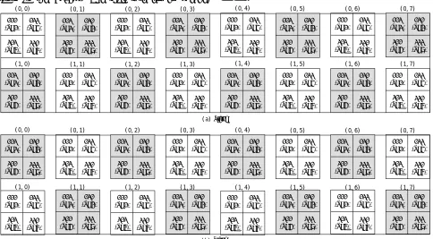
Figure 6 shows the 3-D implementation of DLH(4,3) network using the proposed construction algorithm (figure 8(a) corresponds to PlaneL, and figure 8(b) to
PlaneR). The required connections for the DLH(m,d)
network constructed by the algorithm are as follows. Let
d be the size of a node square. Shifts in the amount of ±
[2×Dr(n)-Dr(n -3)]×d in row-wise direction and ±[2
×Dc(n)-Dc(n-3)×d in column-wise direction accomplish
the required connection for the three-nearest-neighbor links in the DL(2m). Shifts in the amount of ±[2× Dc(n)-Dc(n -3)]×(2m -1)×d in column-wise direction
accomplish the required connection for the wrap-around links in the DL(2m). The shift rule for an n-cube,
ROWHC(n) and COLHC (n) generates required connection for the hypercube links. Thus the shift rule for an DLH(m,d), denoted by ROW DLH, and COLDLH, can be expressed as follows:
ROWDLH= ROWHC(n), ±[2×Dr(n)-Dr(n -3)],
COLDLH = COLHC(n), ±[2×Dc(n)- Dc(n-3)],
±[2×Dc(n)-Dc(n-3)]×(2m -1).
Ascan be seen in figure 6, we can expand the size of the DLH(m,d)by adding more hypercube layouts used as
basic building blocks along the perimeter of the DL(2m).
The number of shifts (number of fan-outs) in the shift rule remains unchanged. This is very desirable feature because the optical interconnect module that generates the required number of shifts and the required amount of each shift remains unchanged even if the network grows in size. 000 (PE0) 111 (PE7) 010 (PE2) 100 (PE4) 001 (PE1) 110 (PE6) 101 (PE5) 011
(PE3) (PE0)000
111 (PE7) 010 (PE2) 100 (PE4) 001 (PE1) 110 (PE6) 101 (PE5) 011 (PE3) 001 (PE1) 111 (PE7) 100 (PE4) 010 (PE2) 000 (PE0) 111 (PE7) 010 (PE2) 100 (PE4) 001 (PE1) 110 (PE6) 101 (PE5) 011
(PE3) (PE0)000
111 (PE7) 010 (PE2) 100 (PE4) 001 (PE1) 110 (PE6) 101 (PE5) 011 (PE3) PlaneL PlaneR ( a) (b) (0, 0) (0, 1) (0, 2) (0, 3)
(1, 0) (1, 1) (1, 2) (1, 3)
(0, 0) (0, 1) (0, 2) (0, 3)
(1, 0) (1, 1) (1, 2) (1, 3)
000 (PE0) 111 (PE7) 010 (PE2) 100 (PE4) 001 (PE1) 110 (PE6) 101 (PE5) 011 (PE3) 000 (PE0) 111 (PE7) 010 (PE2) 100 (PE4) 001 (PE1) 110 (PE6) 101 (PE5) 011 (PE3)
(0, 4) (0, 5) ( 0, 6) (0, 7)
(1, 4) (1, 5) ( 1, 6) (1, 7)
000 (PE0) 111 (PE7) 010 (PE2) 100 (PE4) 001 (PE1) 110 (PE6) 101 (PE5) 011 (PE3) 000 (PE0) 111 (PE7) 010 (PE2) 100 (PE4) 001 (PE1) 110 (PE6) 101 (PE5) 011 (PE3)
(0, 4) (0, 5) ( 0, 6) (0, 7)
(1, 4) (1, 5) ( 1, 6) (1, 7)
001 (PE1) 111 (PE7) 100 (PE4) 010 (PE2) 001 (PE1) 111 (PE7) 100 (PE4) 010 (PE2) 001 (PE1) 111 (PE7) 100 (PE4) 010 (PE2) 000 (PE0) 110 (PE6) 101 (PE5) 011 (PE3) 000 (PE0) 110 (PE6) 101 (PE5) 011 (PE3) 000 (PE0) 110 (PE6) 101 (PE5) 011 (PE3) 000 (PE0) 110 (PE6) 101 (PE5) 011 (PE3) 001 (PE1) 111 (PE7) 100 (PE4) 010 (PE2) 001 (PE1) 111 (PE7) 100 (PE4) 010 (PE2) 001 (PE1) 111 (PE7) 100 (PE4) 010 (PE2) 001 (PE1) 111 (PE7) 100 (PE4) 010 (PE2) 000 (PE0) 110 (PE6) 101 (PE5) 011 (PE3) 000 (PE0) 110 (PE6) 101 (PE5) 011 (PE3) 000 (PE0) 110 (PE6) 101 (PE5) 011 (PE3) 000 (PE0) 110 (PE6) 101 (PE5) 011 (PE3)
Figure 6. DLH(4,3) embedding: (a) PlaneL (b) PlaneR. A pair of (i, j) : address in DL(2m), a binary string of a3a2a1 : address in hypercube.
VI. CONCLUSION
To overcome the lack of scalability in the regular hypercube networks, a new interconnection network topology, called an Double-Loop Hypercube, is presented. The proposed network is a combination of the hypercube and the DL(2m) topologies. The analysis results show
that the new interconnection network is scalable, meaning the configuration of the existing nodes is relatively insensitive to the growth of the network size, and more efficient in terms of communication. It is also shown that the new interconnection network is highly fault-tolerant. Any faulty node or link can be bypassed by only two additional hops with little modification of the fault-free routing scheme. Due to the concurrent existence of multiple the DL(2m) and the hypercube, the new network
provides a great architectural support for parallel processing and distributed computing.
More importantly, the proposed network is highly amenable to optical implementations.Athree-dimensional optical implementation technique of the proposed network is provided. It is based on an efficient three- dimensional space-invariant implementation scheme for the regular hypercube. The proposed optical implementation technique for the new network results in totally space-invariant connection pattern at every node. Consequently, simple and cost-efficient optical implementation of the proposed network with existing optical hardware would be possible.
ACKNOWLEDGEMENT
Foundation of China (90607008) and ASIC design center, Xi'an Institute of Posts and Telecommunications, China.
REFERENCE
[1] Ruei-Yu Wu,Chang, J.G.,Gen-Huey Chen, “Node- disjoint paths in hierarchical hypercube networks”, 20th International
Parallel and Distributed Processing Symposium, 25-29 April 2006,5 pp.
[2] W. D. Hillis, “The Connection Machine”, MIT Press, Cambridge, MA, 1985.
[3] Dally W, Towles B, “Principles and Practices of Interconnection Networks” , Morgan Kaufmann Press, San
Francisco, 2004.
[4] Ananth Grama,Anshul Gupta,George Karypis etc. Introduction to Parallel Computing (Second Edition)[M]. Addison-Wesley Press,2003.
[5] Peter K.K. Loh, Wen Jing Hsu, Yi Pan, “The Exchanged Hypercube”, IEEE Transations on Parallel and Sistributed Systems, Vol. 16, No. 9, Sptember 2005,pp.866-874.
[6] A.Louri, H.Sung, “Scalable Optical Hypercube- Based Interconnection Network for Massively Parallel Computing”,
Applied Optics, vol. 33, Nov. 1994.pp.7588-7598.
[7] A.Louri, B. Weech, C. Neocleous, “A spanning multichannel linked hypercube: a gradually scalable optical interconnection network for massively parallel computing”, IEEE Transactions on Parallel and Distributed Systems, Volume 9, Issue 5, May 1998,pp.497-512
[8] F.P.Preparata and J.Vuillemin, “The cube-connected cycles: a versatile network for parallel computation”, Communications of the ACM, 24(5), 1981, pp.300-309.
[9] Q.M. Malluhi, M.A. Bayoumi, “The Hierarchical Hypercube: A New Interconnection Topology for Massively Parallel Systems”, IEEE Trans. Parallel and Distributed Systems, vol. 5,
no. 1, Jan. 1994,pp.17-30.
[10] W.J. Hsu, M.J. Chung, and Z. Hu, “Gaussian Networks for Scalable Distributed Systems”, The Computer J., vol. 39, no. 5,
1996, pp. 417-426.
[11] S.G. Ziavras, “RH: A Versatile Family of Reduced Hypercube Interconnection Networks”, IEEE Trans. Parallel and Distributed Systems, vol. 5, no. 11, Nov. 1994, pp.
1210-1220.
[12] K. Ghose and K.R. Desai, “Hierarchical Cubic Networks” ,
IEEE Trans. Computers, vol. 6, no. 4, Apr. 1995, pp. 427-435.
[13] J.M. Kumar, L.M. Patnaik, “Extended Hypercube: A Hierarchical Interconnection Network of Hypercubes”, IEEE Trans. Parallel and Distributed Systems, vol. 3, no. 1, Jan. 1992,
pp. 45-57.
[14] N.-F. Tzeng and S. Wei, “Enhanced Hypercubes” , IEEE Trans.Computers, vol. 40, no. 3, Mar. 1991, pp. 284-294. [15] L.N.Bhuyan,D.P.Agrawal,“Generalized Hypercube and Hyperbus Structures Constructing Massively Parallel
Computers”, IEEE Trans. Computers, vol. 33, 1984, pp.
323-333.
[16] C. Chen, D.P. Agrawal, and J.R. Burke, “dBCube: A New Class of Hierarchical Multiprocessor Interconnection Networks
with Area Efficient Layout”, IEEE Trans. Parallel and
Distributed Systems, vol. 4, no. 1, Jan. 1993,pp .332-1,344.
[17] A. Louri and H. Sung, “A design methodology for three-dimensional space-invariant hypercube networks using graph bipartitioning”, Optics Lett., vol. 18, Dec, 1993, pp.
2050-2052.
[18] A. Louri and H. Sung, “Efficient implementation methodology for three-dimensional space-invariant hypercube-based free-space optical interconnection networks,”
Appl. Optics, vol. 32 , Dec. 1993, pp. 7200-7209.
[19] F. Kiamilev, P. Marchand, A. V. Krishnamoorthy, S. C.
Esener, and S. H. Lee, “Performance comparison between optoelectronic and VLSI multistage interconnection networks,”
IEEE J. Lightwave Technol., vol. 9, Dec. 1991, pp. 1665-1674.
[20] R. A. Nordin, A. F. J. Levi, R. N. Nottenburg, J. O’Gorman, T. Tanbun-Ek, and R. A. Logan, “A system perspective on
digital interconnection Technology,” IEEE J. Lightwave
Technol., vol. 10, Jun. 1992, pp. 811-827.
LIU Youyao received the B.E. and M.S. degree in electronics
engineering from Xi’an University of Science & Technology, Xi’an, China, in 2000 and 2003. He is pursuing the Ph.D. at XIDIAN University, Xi’an, China.
He works as a lecturer at Xi'an Institute of Post and Telecommunication. His research interests focus on the area of design and verification of SoC, Parallel computing, etc.
HAN Jungang received the B.E. in Mathematics Department of
Jilin University, China, in 1966 and M.S. in Institute of Computing Technology , Chinese Academy of Science, Beijing, P.R. China, in 1981.
From 1967 to 1975, he worked as a Electronic Engineer, the 795th Factory at Xian Yang, Shaanxi Province, China. From 1982 to 1993,he is an associate professor, XIDIAN University Xi’an China. He is a visiting scholar, Computer Science Department, University of Calgary, Canada, Oct. 1986 to Sept. 1988. Since 1994 he has been on the faculty of the Department of Computer Science at Xi'an Institute of Post and Telecommunication, where he is a professor, director, and doctor tutor of Department of Computer Science.
He is active in formal design and verification of SoC, application technology of computer etc. He has published numerous journal and conference articles. From 1999, Professor HAN received Chinese Government special subsidy,. He is a senior member of member of Chinese Computer Federation, Chinese Communication Federation, special committee of CAD&CG, CCF.
DU Huimin received the M.S. and PhD degree in computer
science XIDIAN University, China, in 1992 and 2000. From 2000 to 2002, she got a postdoctoral position in Northwestern Polytechnical University , Xi'an , China.