A Visual Words Selection Strategy for Pedestrian
Detection and Analysis of the Feature Points Distribution
Xingguo Zhang
1*, Guoyue Chen
2, Kazuki Saruta
2, Yuki Terata
21 Graduate School of Systems Science and Technology, Akita Prefectural University, Japan.
2 Faculty of Systems Science and Technology, Akita Prefectural University, Japan.
* Corresponding author. Tel.: +81-174-27-2087; email: [email protected] Manuscript submitted July 28, 2014; accepted October 10, 2014.
doi: 10.17706/jcp.10.1.57-67
Abstract: An effective and efficient visual word selection method based on Bag-of-features (BoF), which can be applied to the pedestrian detection problem, is proposed in this paper. We first calculate the difference in the total appearance frequency of each visual word in pedestrian and non-pedestrian images. Visual words that exhibit greater absolute values are more efficient for pedestrian detection, and are thus selected. The effectiveness of the proposed method is validated by analyzing the distribution of selected feature points. Through this analysis, we find that discriminative feature points for pedestrian images are mainly located about the lower body, whereas those for non-pedestrian images are mainly located in background areas. Experimental results show that, using the proposed method, the detection rate for the Daimler-DB datasets exceeds 92.5%, whereas the miss rate is less than 6.8%. More-over, the time required for learning and detection can be reduced by approximately 50%, with no significant degradation in precision, using the proposed method, even if only 40% of the visual words are selected.
Key words: Bag-of-features, visual words selection, pedestrian detection, feature points distribution.
1.
Introduction
Over the past twenty years, research has moved toward intelligent systems that predict dangerous situations and anticipate accidents [1], [2]. These are known as advanced driver assistance systems, in the sense that they help the driver by providing warnings, assisting in decision-making, and even automatically taking evasive action. However, many challenges remain, especially the rapid, high-precision detection of pedestrians.
The simplest technique for determining the initial location of an object is the sliding window method, whereby detector windows at various scales and locations are shifted over the image. However, the computational cost of high-precision detection in every sliding window is often too high to allow for real-time processing [3]-[5]. To speed up the process, pedestrian detection is often decomposed into a two-stage procedure to reduce the search area. First, the system defines a region of interest (ROI), which is possibly associated with a potential pedestrian. The Haar wavelet-based cascade framework [6] is a powerful tool for ROI selection, and can be combined with AdaBoost [7] to construct a classifier. Second, detection is validated by a high-precision identification method for the ROI. However, this process also suffers from certain limitations, particularly when the pedestrian is not positioned in the middle of the ROI search window.
characterized by local visual descriptors. These are quantized by vectors using the clustering algorithm (e.g. K-means) to produce so-called visual words [8], [9]. The introduction of such visual words has allowed significant advances in image classification, especially when combined with bag-of-features (BoF) models [10]. One advantage of BoF is that the frequency histogram is independent of the location of the local feature, and is very useful in detecting the image of a pedestrian under a position shift. Although not every visual word created by K-means leads to an efficient classification, compact visual codebooks present advantages in both computational efficiency and memory usage.
A compact and discriminative visual vocabulary has been proposed by [11]. Their approach hierarchically merges the visual words in a large initial vocabulary, and requires the new histograms to maximize the conditional probability of the true labels of the training images. This is a rigorous but complicated criterion that involves nontrivial computation after each merging operation. Consequently, this method has a heavy computational load when dealing with large-sized initial visual words.
Many visual word selection methods have subsequently been proposed [12], [13], but it seems to be difficult to achieve both speed and good discrimination.
In this paper, we consider two-class classification problems, and propose a very simple method to reduce the dimension of the classifier by setting a limit value to remove irrelevant and redundant visual words. Our method calculates the difference in the total appearance frequency for each visual word of the pedestrian and non-pedestrian images. The visual words that exhibit greater absolute values are considered to be more efficient for pedestrian detection, and are selected. Experimental results show that the proposed method retains almost the same detection accuracy when only 40% of the visual words are selected.
In the remainder of this paper, we first introduce the process of pedestrian detection using the BoF method, before describing our approach and presenting experimental results and conclusions.
2.
Pedestrian Detection Based on BoF
In this section, we describe the process of pedestrian detection using a BoF approach, and examine some existing problems. BoF is an object classification method that ignores the positional information of the local features extracted from the images, and uses the occurrence frequency histogram of visual words as the training data to construct a classifier.
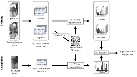
Fig. 1 shows the basic flowchart of BoF pedestrian detection, which consists of a training stage and a testing stage. In the training stage, local features are extracted from the training samples, and are clustered into a number of groups by some clustering algorithm. After clustering, the visual vocabulary is built, and the frequency histogram of each visual word is calculated. The frequency histogram derived from the visual vocabulary is considered to be the input classifier, and this is trained by some machine learning algorithm. In the recognition stage, the frequency histogram of local features extracted from the test samples is calculated in the same manner, and the constructed classifier makes decisions based on this frequency histogram.
Typical machine learning methods include decision tree learning, artificial neural networks (ANN), support vector machines (SVM), etc. In our experiments, we use SVM because it is effective when the training data consists of a small number of samples in high-dimensional spaces.
Details of each process are described below.
2.1.
Local Feature Extraction
on interest point feature extraction. SIFT can robustly identify objects even among clutter and under partial occlusion, because the SIFT feature descriptor is invariant to uniform scaling, orientation, and partially invariant to affine distortion and illumination changes. However, SIFT needs to structure the Gaussian scale space to find interest points, and therefore cannot always extract enough features for low-resolution pedestrian images.
Fig. 1. Pedestrian detection process of BoF.
To obtain better discriminative power, we utilize a regular dense sampling method, known as dense-SIFT descriptors. This is roughly equivalent to running SIFT on a dense grid of locations at a fixed scale and orientation, but without the need to structure the Gaussian scale space to find interest points.
2.2.
Forming the Visual Vocabulary and Frequency Histograms
Various clustering methods can be used to form the visual vocabulary, such as k-means [16], affinity propagation [17], self-organizing maps [18], fuzzy c-means [19], etc. Each method has its strengths, but inevitably has some weaknesses. In terms of a combination of efficiency and accuracy, k-means is a satisfactory clustering method.
Visual vocabularies are created as follows. After extracting a large number of local patch descriptors (here, dense-SIFT descriptors) from a set of training images, k-means clustering is used to group these descriptors into k clusters, where k is predefined. The center of each cluster is called the “visual word,” and a set of visual words forms a “visual vocabulary.” Each image descriptor is then labeled with the most similar visual word, according to the Euclidean distance between the two, and the image is characterized by a k-dimensional histogram of the number of occurrences of each visual word. The frequency histogram of each visual word forms the training data that is input to the SVM.
2.3.
SVM Classifier
SVM is a well-known statistical learning method [20]. The objective of SVM learning is to find a hyperplane that maximizes the inter-class margin of the training samples. Feature vectors are projected into a high-dimensional space by a kernel function. The final SVM classifier is given by the following expression. T ra in in g R ec o g n it io n Test image input positive Training images input
Output: person vs. non-person (a) Local features
extraction
W2 W7…W6
W1 W5…W9
……
W2 W7…W6
W1 W5…W9
……
W2 W7…W6
W1 W5…W9
……
W5 W6…W9
W2 W3…W7
……
W5 W6…W9
W2 W3…W7
……
W5 W6…W9
W2 W3…W7
……
W2 W6…W8
W3 W5…W9
……
(b) clustering negative
i
, i
if x
K x x (1)where are support vectors and is the kernel function. There are several common kernel
functions, such as a linear kernel, polynomial kernel, radial basis function (RBF) kernel [21], etc. The choice of kernel function is dependent on the data and application. We tested each kernel function, and found that an RBF kernel gives the best performance without any obvious deterioration in efficiency. Thus, in our experiments, we use an RBF kernel.
3.
Overview of Our Approach
One disadvantage of the dense regular grid is that a large number of redundant features are included in the visual vocabulary, meaning more time will be spent on feature extraction and classification during the training and recognition stage. A simple and efficient visual vocabulary is expected to speed up learning and classification. Hence, we propose a method to reduce the dimension of the classifier by setting a limit value to remove irrelevant and redundant visual words.
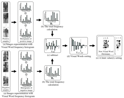
Fig. 2. Flowchart of proposed method.
A brief overview of this approach is given in Fig. 2. First, the quantization histograms obtained from each training image are divided into positive images and negative images (Fig. 2(a)). The total frequency
histograms for positive sample and negative sample are then computed by the following equation,
as shown in Fig. 2(b).
1, , 1, , 1 0 i i N x Xi j M x X
H x h
H x x h x
(2)
√ ×
L
x xL
L
Positive samples
(a) Images representation with Visual Word frequency histogram
Negative samples Histograms of positive image Visual Word fr eq u en cy H (c) subtract Vdiff x Vsort_diff x L
(d) Visual Words sorting
(e) A limit value(L) setting
New Visual Word Dictionary Visual Word fr eq u en cy 1 H0 Visual Word fr eq u en cy Visual Word fr eq u en cy Visual Word fr eq u en cy Histograms of negative image Visual Word fr eq u en cy Visual Word fr eq u en cy Visual Word fr eq u en cy
(a) Images representation with Visual Word frequency histogram
(b) The total frequency calculation
T1 1 1
T
0 1 1 1
:
:
0 , 1 ,...,
0 , 1 ,...,
H H H X
H H H X
1
H
H
where X is the number of visual words in a dictionary. N and M represents the number of pedestrian and
non-pedestrian training samples, respectively. represents the frequency of x’th visual word on i’th
pedestrian image. represents the frequency of x’th visual word on j’th non-pedestrian image.
Next, we normalize the two total frequency histograms as
1 11
0 0
1
0 1
X x
X x
H x H x
H
H x
H x
H x
x
(3)
The difference between and is calculated to obtain the difference vector (Fig. 2(c))
= 1
0
diff
V x H x H x (4)
If is positive, this visual word is effectively classified as a positive sample, and vice versa.The
larger the absolute value of , the more beneficial the x-th feature to the classification.
The visual words are sorted in descending order of absolute value, and a limit value L is set to determine
the expected size of the new visual vocabulary to be preserved (Fig. 2(d)). Visual words for which
is below the limit value L are considered to be redundant, and are screened out of the original dictionary.
The remaining L visual words comprise a new visual vocabulary (shown in Fig. 2(e)). Next, the
corresponding dimensions of the original histograms are removed according to the new visual
vocabulary. The new frequency histogram of the visual vocabulary forms the input to the classifier, which is trained by the SVM.
4.
Experimental Results
In this section, we evaluate the performance of our proposed method in terms of its detection rate and processing time. In addition, we analyze the distribution of discriminative features by visualizing the selected features. We implement our proposal method using Matlab, and use the open-source toolbox VLFeat [22] to extract SIFT features and form the visual vocabulary. We use the LibSVM [23] to train the classifier, which is integrated software for support vector classification.
4.1.
Experimental Conditions
We used the Caltech Pedestrians [24], DaimlerChrysler Pedestrian Classification Benchmark (Daimler-CB) [25], and Daimler Pedestrian Detection Benchmark (Daimler-DB) [26] datasets to conduct a series of experiments.
These datasets were collected by the on-board camera within a vehicle, and include images of pedestrians from different viewpoints.
In our experiments, we applied training to these three datasets, and created the detectors respectively. The sizes of both the training and test images were uniformly fixed at 48 × 96 pixels.
We sampled SIFT features densely over 4-pixel intervals, with a block size of 8 × 8 pixels. This results in 256 SIFT feature points being extracted from each 48 × 96 pixel sample. Using the dense-SIFT feature
visual vocabulary. The SVM detectors were then trained using RBF kernels. The performance of SVM
classifier depends on the choice of the regularization parameter C and the kernel parameters . We use the
grid search with cross-validation to determine the optimal values of the parameters C and . Experimental
results show that the classifier attains optimal performance when C = 16 and .
4.2.
Detection Accuracy with Various Sizes of Visual Vocabulary
To clarify the relationship between the detection accuracy and the size of the visual dictionary, and determine the initial number of visual words in the proposed method, we conducted the following experiment.
We randomly selected 3000 pedestrian and 3000 non-pedestrian images from the Caltech, Daimler-CB, and Daimler-DB datasets as the training samples. For the test samples, 3000 pedestrian and 3000 non-pedestrian images were selected from the remainder of each dataset.
We varied the size of the initial visual vocabulary X from 200 to 2000, and tried to ascertain the optimal
value for each dataset. The detection accuracies for different X are shown in Fig. 3.
The results in Fig. 3 show that optimal detection accuracy of each dataset is achieved when X is around
500. Thus, in the following evaluations, the initial number of visual words X is set to 500.
Daimler-CB Daimler-DB Caltech
Fig. 3. Relation between visual word X and detection precision.
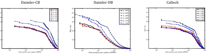
Daimler-CB Daimler-DB Caltech
Fig. 4. Relation between limit value L and detection precision.
4.3.
Detection Accuracy with Various Sizes of Selected Visual Word
In this section, we describe the relation between the limit size L of the visual vocabulary and the
detection accuracy for the three datasets.
Using an initial visual vocabulary size X = 500 for training and testing images, the value of L was varied
from 400 to 100. The detection accuracy at different L values is shown in Fig. 4. The results show similar
results for the three datasets, with small variations in accuracy when L ≥ 200. This implies that 200 efficient
visual words in the original visual vocabulary produces almost the same performance as using all 500 visual
words. In addition, the detection precision decreases more quickly when L < 200.
10-3 10-2 10-1 100 0.1 0.2 0.3 0.5 0.7 0.9
False positives per window (FPPW)
M is s rat e X=200 X=300 X=400 X=500 X=700 X=1000 X=2000
10-3 10-2 10-1 100 0.1 0.2 0.3 0.5 0.7 0.9
False positives per window (FPPW)
Mi ss rat e X=200 X=300 X=400 X=500 X=700 X=1000 X=2000 10-3 10-2 10-1 100 0.1 0.2 0.3 0.5 0.7 0.9
False positives per window (FPPW)
M is s ra te X=200 X=300 X=400 X=500 X=700 X=1000 X=2000 10-3 10-2 10-1 100 0.1 0.2 0.3 0.5 0.7 0.9
False positives per window (FPPW)
M is s ra te L=500 L=400 L=300 L=200 L=150 L=100
10-3 10-2 10-1 100 0.1 0.2 0.3 0.5 0.7 0.9
False positives per window (FPPW)
Mi ss rat e L=500 L=400 L=300 L=200 L=150 L=100 10-3 10-2 10-1 100 0.1 0.2 0.3 0.5 0.7 0.9
False positives per window (FPPW)
These results show that the proposed method retains similar detection accuracy when only 40% of the
visual words are selected. Thus, we can set L = 0.4X without significantly affecting the accuracy.
4.4.
Evaluation of Pedestrian Detection by Cross Experiments
In this section, we evaluate the proposed method for pedestrian detection using the following cross
experiment. First, we set X = 500 and L = 200. We randomly selected 3000 pedestrian images for Groups A
and B, and 3000 non-pedestrian images for Groups C and D from the Daimler-DB dataset. Different combinations of these groups were then used to perform the cross experiment.
Table 1. Evaluation of the Proposed Method
Training Data Test Data True Positive False Positive Training Data A C
A D B C B D
B D B C A D A C
92.8% 92.5% 93.1% 92.6%
6.3% 6.6% 6.0% 6.8%
A C A D B C B D
Table 1 shows the experimental results. We found that the detection rate for each group was greater than 92.5%, and the miss rate was less than or equal to 6.8%. This confirms that the proposed method is effective for pedestrian detection applications.
4.5.
Visualization of the Discriminative Feature Points
We now analyze the distribution of selected feature points from pedestrian and non-pedestrian images, and present the average number of discriminative features in the pedestrian images. In addition, we discuss the causes of false positive (FP) and false negative (FN) results.
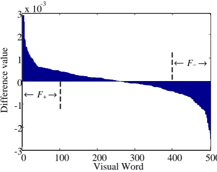
Fig. 5. Justification of and with visual words.
Fig. 5 shows the result of sorting the difference vector obtained from the process in Fig. 2(d) with an
initial visual dictionary size X = 500. The horizontal axis represents the number of visual words, and the
vertical axis represents the difference in the total occurrence frequency of each visual word between the pedestrian and non-pedestrian images. Visual words for which the difference is positive are considered to contribute to the determination of pedestrians, whereas negative values imply that the visual word contributes to the determination of non-pedestrian objects. As shown in Fig. 5, we defined the top 100
visual words for determining pedestrians as , and the 100 visual words that best represent
non-pedestrian objects as .
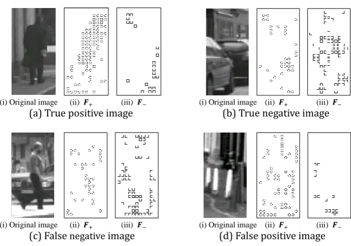
Fig. 6 illustrates examples of the distribution of (‘○ ’ in the figure) and (‘□ ’ in the figure) in the
0 100 200 300 400 500
-3 -2 -1 0 1 2 3x 10
-3
Visual Word
D
if
fe
re
n
ce
v
al
u
e
F+
case of true positive (TP), true negative (TN), FN, and FP detections.
In the pedestrian images in Fig. 6(a), it can be see that feature points are mainly located about the
body, whereas are mainly located in the background. In the rejected non-pedestrian image shown in Fig.
6(b), the distribution of feature points varies widely, but there are many more feature points than .
In the FN image in Fig. 6(c), the points are again mainly located about the body, but there are fewer
than in the TP image. We suspect this is because FN images have complicated backgrounds, which will affect
the detection accuracy. In contrast, in the FP image, the points are in the majority, and so this image was
determined to contain a pedestrian.
(i) Original image (ii) (iii) (i) Original image (ii) (iii) (a) True positive image (b) True negative image
(i) Original image (ii) (iii) (i) Original image (ii) (iii) (c) False negative image (d) False positive image
Fig. 6. Visualization of selected feature points.
4.6.
Processing Time Performance
In this section, we study the relationship between the processing time and the number of selected visual
words L. We compare the SVM runtime on the same desktop with an Intel i3-540 CPU and 2 GB RAM.
Fig. 7. Change in recognition time with L using 6000 images.
Fig. 7 shows that the recognition time increases with the value of L for 6000 images. As mentioned above,
the detection accuracy is not obviously reduced as L is decreased to 200. Thus, the experimental results
show that the classification time required by the SVM can be reduced by about 50% using the proposed method, without any significant degradation in accuracy, even if only 40% of the visual words are selected.
100 200 300 400 500
0 20 40 60 80
Selected Visual Word
Reco
g
n
it
io
n
t
ime(s
)
8
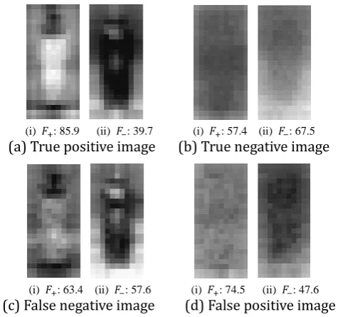
(i) : 85.9 (ii) : 39.7 (i) : 57.4 (ii) : 67.5 (a) True positive image (b) True negative image
(i) : 63.4 (ii) : 57.6 (i) : 74.5 (ii) : 47.6 (c) False negative image (d) False positive image Fig. 8. Average distribution and number of selected features.
4.7.
Average Distribution of the Selected Feature Points
In this section, we analyze the average distribution of selected feature points from TP, TN, FN, and FP images.
We randomly selected 500 correctly classified pedestrian and non-pedestrian images for the TP and TN dataset, and 500 incorrectly classified pedestrian and non-pedestrian images for the FN and FP dataset from the classification results of Section 4.4. We then examined the average number of selected discriminative features of each set.
To compare the difference in the feature point distribution of pedestrian and non-pedestrian images, we divided each detection window into 11 × 22 grids, and computed the average number of feature points in each cell.
Fig. 8 shows the average distribution of and feature points in TP, TN, FN, and FP image sets. The
white area indicates a large number of feature points in the figure, and the black area indicates the opposite.
The figure shows that, for pedestrian images (TP or FN), feature points are mainly located about the
body, and points are primarily in the background. This is because features located in the background
are highly consistent with those extracted from non-pedestrian images. In the non-pedestrian images (TN
or FP), both and are uniformly distributed in the images. This is because the position of
changes with the content of the non-pedestrian images.
Furthermore, in the pedestrian images, are mainly located in the lower body areas. We speculate that
this is because, in pedestrian images, feature points located around the shoulder areas suffer more interference with the background, so the discriminative features are mainly distributed in the lower part of the body.
Fig. 8 also shows the average number of selected discriminative feature points for each image set. It can
be seen that the average number of points in TP images (85.9) far outweighs that of (39.7), but in
the TN images, the number of points (67.5) outweighs that of (57.4). This is the greatest difference
between the TP and TN images. In contrast, in the FN images, the count of (63.4) is close to (57.6),
whereas in the FP images, (74.5) far outweighs (47.6).
Overall, it can be said that the number of discriminative features is a significant factor in the detection
accuracy. Furthermore, an unknown image can be determined to contain a pedestrian when the count
non-pedestrian image.
5.
Conclusion
This paper presented a method of obtaining a compact and discriminative visual vocabulary for pedestrian detection. Our visual word selection method calculates the difference in the total appearance frequency of each visual word in pedestrian and non-pedestrian images. The visual words that exhibit greater absolute values are considered to be more efficient for pedestrian detection, and are thus selected. In addition, we investigated the distribution of discriminative feature points belonging to the selected visual words from pedestrian images and non-pedestrian images. As shown by the experimental results, discriminative feature points in the pedestrian images are mainly located in body areas, whereas the feature points are uniformly distributed in non-pedestrian images. The experiments also showed that the learning and detection process can achieve similar precision in about 50% of the time using the proposed method, even if only 40% of the visual words are selected. In future work, more theoretical and experimental studies will be conducted to analyze the performance of our method.
References
[1] Yan, J., Zhang, X., Zhen, L., Liao, S., & Li, S. Z. (2013). Robust multi-resolution pedestrian detection in
traffic scenes. Proceedings of IEEE Int’l Conf. on Computer Vision and Pattern Recognition (pp.
3033–3040).
[2] Dollar, P., Wojek, C., Schiele, B., & Perona, P. (2012). Pedestrian detection: An evaluation of the state of
the art. IEEE Trans. Pattern Analysis and Machine Intelligence, 34, 743–761.
[3] Dalal, N., & Triggs, B. (2005). Histograms of oriented gradients for human detection. Proceeding of IEEE
Computer Society Conf. on Computer Vision and Pattern Recognition: Vol. 2 (pp. 886–893).
[4] Wu, B., & Nevatia., R. (2007). Detection and tracking of multiple, partially occluded humans by Bayesian
combination of edgelet based part detectors. Int’l J. Computer Vision, 75, 247–266.
[5] Sabzmeydani, P., & Mori, G. (2007). Detecting pedestrians by learning shapelet features. Proceedings of
IEEE Int’l Conf. on Computer Vision and Pattern Recognition (pp. 1–8).
[6] Viola, P., Jones, M., & Snow, D. (2005). Detecting pedestrians using patterns of motion and appearance.
Int’l J. Computer Vision, 63, 153–161.
[7] Freund, Y., & Schapire, R. E., (1997). A decision-theoretic generalization of on-line learning and an
application to boosting. J. of Computer and System Sciences, 119–139.
[8] Sivic, J., & Zisserman, A. (2003). Video Google: A text retrieval approach to object matching in videos.
Proceedings of IEEE Int’l Conf. on Computer Vision: Vol. 2 (pp. 1470–1477).
[10]Csurka, G., Dance, C., Fan, L., Williamowski, J., & Bray. C. (2004). Visual categorization with bags of
keypoints. Proceedings of European Conf. on Computer Vision (pp. 59–74).
[11]Winn, J., Criminisi, A., & Minka. T. (2005). Object categorization by learned universal visual dictionary.
Proceeding of IEEE International Conf. on Computer Vision: Vol. 2 (pp. 1800–1807).
[12]Wang, L., Zhou, L., & Shen, C. (2008). A fast algorithm for creating a compact and discriminative visual
codebook. Proceedings of European Conf. on Computer Vision (pp. 719–732).
[13]Moosmann, F., Triggs, B., & Jurie, F. (2007). Fast discriminative visual codebooks using randomized
clustering forests. Proceedings of Advances in Neural Information Processing Systems (pp. 985–992).
[14]Lowe, D. G. (2004). Distinctive image features from scale-invariant keypoints. Proceeding of IEEE Int’l
Conf. on Computer Vision: Vol. 60 (pp. 91–110).
[9] Uijlings, J. R. R. A., Smeulders, W. M., & Scha, R. J. H. (2010). Real-time visual concept classification. IEEE
[16]Hartigan, J. A., & Wong, M. A., (1979). A K-means clustering algorithm. Applied Statistics, 28, 100–108.
[17]Frey, B. J., & Dueck, D. (2007). Clustering by passing messages between data points. Science, 315,
972–976.
[18]Kohonen, T., et al. (1982). Self-organized formation of topologically correct feature maps. Biological
Cybernetics, 43, 59–69.
[19]Ahmed, M. N., Yamany, et al. (2002). A modified fuzzy C-means algorithm for bias field estimation and
segmentation of MRI data. IEEE Trans. Medical Imaging, 21, 193–199.
[20]Vapnik., V. (1995). The Nature of Statistical Learning Theory. Springer-Verlag.
[21]Cao, N. H. T., & Ninomiya, Y. (2008). Approximate RBF kernel SVM and its applications in pedestrian
classification. MLVMA’08.
[22]VLFeat. From: http://www.vlfeat.org/
[23]LIBSVM — A Library for Support Vector Machines. From: http://www.csie.ntu.edu.tw/~cjlin/libsvm/
[24]Dollar, P., Wojek, C., Schiele, B., & Perona, P. (2009). Pedestrian detection: A benchmark. Proceeding of
IEEE Conf. on Computer Vision and Pattern Recognition (pp. 304-311).
[25]Munder, S., & Gavrila, D. M. (2006). An experimental study on pedestrian classification. IEEE Trans.
Pattern Analysis and Machine Intelligence, 28, 1863–1868.
[26]Enzweiler, M., & Gavrila, D. M. (2009). Monocular pedestrian detection: Survey and experiments. IEEE
Trans. Pattern Analysis and Machine Intelligence, 31, 2179–2195.
Xingguo Zhang received the B.Sc. degree in computer science from the Dalian Polytechnic University of China in 2009, and the M.Sc. degree from the Akita Prefectural University of Japan in 2012. He is currently working toward the PhD degree with the project “Pedestrian detection in advanced driver assistance systems”. His research interests include computer vision, pattern recognition, and machine learning.
Guoyue Chen received the B.S. degree from East China Normal University, China, in 1983, where he worked as a research associate at the Department of Computer Science until 1989. He received the M.S. and Ph.D. degrees from Tohoku University, Japan, in 1993 and 1996, respectively. Currently, he is a professor in Akita Prefectural University, Japan. His interests include digital signal processing and its applications to active noise control, and image processing.
Kazuki Saruta received his B.S. and M.S. degrees from Akita University, Japan, in 1991 and 1993, and his Ph.D. degree from Tohoku University, Japan, in 1996, respectively. Now he is an associate professor in Akita Prefectural University, Japan. His research interests include computer vision, machine learning, pattern recognition and information network system.
Yuki Terata received the B.S. degree form Akita University, Japan, in 1998, the M.S. and Ph.D. degrees from same university, in 2000 and 2008. Currently, he is a research associate in Akita Prefectural University, Japan. His research interests include wireless network communication, computer vision, and bionics.
[15]Bay, H., Tuytelaars, T., & Gool, L. V. (2006). Surf: Speeded up robust features. Proceedings of European