A Model for Pricing Insurance Using Options

SCITECH

RESEARCH ORGANISATION

Journal of Research in Business, Economics and Management

www.scitecresearch.com

A Model for Pricing Insurance using Options

S. Dakurah

, F.N.D. Odoi

, B.K. Kongyir

, M.O. Ampaw-Asiedu

and V. K. Dedu

1,2,4,5_{Department of Mathematics, Kwame Nkrumah University of Science and Technology, Kumasi.} 3_{St. Francis Xavier Minor Seminary, Wa.}

Abstract

:

Traditional Expected Value and Bayesian Methods of pricing insurance products are not robust both under minimal data and frequent portfolio adjustments. Deriving a partial differential equation for the price of an insurance put, parallel is struck with the reverse Black Scholes partial differential equation for pricing call options. With appropriate parameter translation of the Black Scholes model, a Pure Premium valuation function that is an improvement over the traditional methods of pricing insurance products results. Its robustness is illustrated with the pricing of a third-party insurance product for private cars.

Keywords:

1

Introduction

The dynamic and unpredictable nature of risk requires innovation and pragmatism in pricing insurance for various risk portfolios. Insurers and underwriters are constantly looking for new pricing methods that are efficient, flexible and can be explained on an intuitive level to the target market.

Insurance is a contract whereby one party, known as the insurer, undertakes, in return for an agreed consideration(premium), to pay a sum of money or its equivalent to the other party, the insured, on the happening of a specified event.

The consideration paid by the insured in exchange for the promised indemnity by the insurer on the happening of the specified event is the Premium.

A derivative is a financial instrument whose value depends on the value of an underlying asset.

An option is a derivative contract conferring on the holder the right to give an asset in exchange for another.

The pricing of financial derivatives is efficient due to the completeness of the financial market and a whole array of robust pricing models and theories.

Pricing of insurance, however, is be-leagued with a plethora of inefficiencies. The application of financial theories to the insurance underwriting process could thus, prove instrumental in translating the stated benefits to the insurance pricing process. This paper sought to develop a pricing model that incorporates the resilience and efficiency of the Insurance and Financial Markets respectively.

The applicability of the model is tested by pricing a Third-Party Insurance for private cars. To achieve this, secondary data was obtained from the Insurance Regulatory and Development Authority of India (IRDAI) and was analyzed with the help of custom-written programs using Visual Basic for Application(VBA) and the Python Programming Language.

2

Method

2.1

Assumptions

a) Completeness. That is, there is negligible cost of effecting insurance, perfect information of the insurance market and equilibrium prices.

b) The insurance market is regulated particularly with respect to equity holdings and reserves.

c) Policy issued is of a short duration with maximum length of 1 year.

d) We also made the simplifying assumption that, all claims incurred during the period are settled at policy expiration.

e) All policies are subject to a deductible amount not less than zero.

2.2

Pure Premium Model

Written exposures usually have the risk unit as the underlying asset. As the policy duration closes in, the price paid for covering that risk unit should reduce correspondingly. The idea being that, the chance of a written exposure resulting in a claim diminishes with decreasing policy period.

If we define p(x,t) to be the present value of premiums of a single policy issued at time t on an exposure with value x

covering a period of T − t.

Then we assume there exists enough shareholder funds at least to the tune of x. If we map out from the shareholder funds, exactly that liability value x, we can assume we have taken a long position in x. This assumption is quite debatable but serves good given our regulated market assumption.

To hedge this position, the firm will need to purchase insurance puts. This creates a hedged position for the insurance firm and will be independent of the value of the exposure.

If we denote the change in the insured value as ∆x, for a small change, we can make the assumption that, the ratio of the change in written premium to change in the insured value is approximately equal to p1 (x,t).

) (1)

The number of additional insurance puts to hold to still keep the hedged position is ∆x. Thus, a change in the insured

value will be approximately offset by a change in the value of the insurance puts.

With the changing values of x and t, if the hedged portfolio is maintained continuously, the above assumptions become certain. Even if the hedged position is not maintained continuously, the risk is fairly small and can easily be diversified away by forming a large portfolio of similar hedged positions.1

mapped-out amount of value x and Since the hedged position contains a

policies, the value of reserve is:

(2)

Change in value of the reserve in a short period is:

(3)

Assuming written premiums are changed continuously, applying stochastic calculus; ∆p(x,t) which is p(x + ∆x,t + ∆t) − p(x,t)

(4)

Where σ2 is the variance rate of return on the mapped-out funds.

Substituting (3.4) into (3.3)

(5)

Assuming return on reserve in the hedge position is certain and equal to r∆t, change in reserve thus must equal the value of reserve times r∆t.

) (6)

This is a similar equation arrived at by Black and Scholes but under different pricing motivation. The solution to this differential equation will give us the pure premium of an insurance policy. Inferring from Black and Scholes;

) (7)

2.3

Parameter Estimation

Having determined the Pure Premium model, it now stands to estimate the parameters of this model.

The ’insurance volatility’ parameter σ is probably the most important input in the model.

The three known methods of estimating this parameter are the historical, implied and local method. Historical as the name implies uses previous occurrence as an estimate of future outcome. Though the past does not always exactly reflect the future, this estimate still serves as a good proxy for volatility. It is also worth mentioning that the historical volatility estimation requires a good amount of data to make statistical sense of the estimate.

On the other hand, Implied volatility simply regress the other parameters on the volatility variable. This require relatively few data as it basically depends on the accuracy of the other estimated variables.

In this paper, we will estimate the historical volatility parameter as a proxy of the insurance volatility.

Various research work has made great strides in providing guidelines as to how this will be estimated. Significant among them is a 2002 research paper;” An Examination of Insurance Pricing and Underwriting Cycles” by Chris K and Hal W of the Warren center for Actuarial Studies and Research. Drawing insights from this paper, we establish the following as an estimate of the ’insurance volatility parameter’.

Let CoV be the coefficient of variation of loss amounts.

This will be used as the standardized measure of riskiness.

The reason been that; the riskier a cash-flow, the higher its coefficient of variation and vice-versa. If we let St+h and St represent the value of the mapped out funds at time t + h and t respectively, then the continuously compounded ’loss

return’ for the interval [t,t + h] is

The standard deviation of ’loss returns’ is given by;

We define It to be the standardized market price of risk at time t.

= standard deviation of equity option price returns over t time period.

We will use the Chicago Board Options Exchange(CBOE) volatility index or VIX as a proxy for St as measured by the S & P 500 index.

Relating this standardized market price of risk to the standardized measure of riskiness, the ’insurance historical volatility parameter’ slosst is given by:

slosst = ItCoV loss (8)

Adjusting the Pure Premium model with these parameters;

2.4

Construction of Portfolio

The Pure Premium determined by equation (3.7) is a” stand-alone” premium and will be quite high. We therefore incorporate the process of portfolio construction to our model, to reduce the pure premium churned out by our model.

This will be a pool of insurance policies with varying risk characteristics. We will determine the total fund amount out of which we will obtain the portfolio savings.

We will also propose a fair way of allocating this portfolio savings to each individual policyholder. We defined the following variables to help establish the mathematical framework for the portfolio construction:

yi = number of written exposures in a portfolio.

nLi_j = the discounted expected loss amount of the j_th exposure in the i_th portfolio with claims frequency of n.

Pij = the jth exposure in portfolio i.

= total expected loss of portfolio i.

St i,j

= past claim amount of the jth exposure in the ith portfolio at time t(with increment one) We make a special provision that, n = 1 plus time lag between first and last claim.

= total loss variation of portfolio i.

= claims variation of the jth exposure.

Total portfolio standard deviation = σLi =

p

PA = Portfolio Amount. PA = φ−1 (0.99) ∗σLi +

P yi Li_j

Total Savings Amount = SA = Pyi Vc − PA

SA will represent the 1% of losses not covered by the written premiums. Let = savings amount of the jth exposure in portfolio i.

Before we adjust the pure premium model with the savings amount, we will account for the other components of the pricing function. Let:

• Ea = ’Additive expenses’

• Em = ’Multiplicative expenses’

• Pa = ’Additive profit margin’

• Pm = ’Multiplicative profit margin’

These are defined per exposure and expenses could be either allocated or unallocated.

We define Pj to be the ’final’ premium of the jth exposure considering expense and profit margins as well as savings amount.

3

Analysis And Discussions

In this chapter, we will walk through the processes involved in sorting the data through to the final pricing of the insurance product.

All claims data used in this study were obtained electronically from IRDAI. These are transactional level data. Claims are aggregated over a period of 8 years.

3.1

Modeling Data

Having chosen to run test our model on Auto insurance, we required individual claim records for this class of insurance as well as stock price returns from CBOE for estimating the parameters of our model. IRDAI collects transactional level data on auto insurance aggregated and grouped into these three broad coverage areas:

a) Third Party Liability Insurance.

b) Collision Coverage.

c) Comprehensive Coverage

We first grouped the claims based on the coverage types above.

Third Party Liability Insurance premium was estimated in our final analysis as claim records on this class was large enough for many realistic estimates.

Having chosen third party, we grouped claims of this coverage type into near homogeneous groups, that is, claims with roughly the same risk characteristics. These groups were then harmonized into risk portfolios.

By doing so, we would have eliminated any abnormal claim amounts. This is not to say losses of disproportionately large sizes won’t occur, but by their nature, we safely ignored their impact on our model and only allow that to the underwriting actuary to deal with as experience may have informed. With our data well sorted, we can proceed to build our model.

3.2

Individual Claims Generation

The claims records were obtained in aggregate form. Our first task was to generate individual claims corresponding to claim occurrence over a period of one year.

Pj = ( jV s

c + Pa + Ea )

(1 − Em ) ∗ (1+ Pm ) , where jV s

For this paper, we generated one hundred and thirty (130) claim records out of the five thousand, eight hundred and thirty-nine aggregated third party (private car) claim records. The outcomes are the time of claim occurrence to payment denoted as ’Time Band’ and the resulting claim amount.

Having obtained the claim amounts and the time bands, we now fit a probability model to these samples.

4

Fitting a Probability Model

In this section, we fit a probability distribution to the generated claim records. Knowing the probability distribution to which claim records originate is of utmost importance to the underwriting actuary in modeling those claims. We demonstrate this distribution fitting process and show how this can be very useful in predicting future claims in the next section.

4.1

Claims

The first thing we did was to plot the claim amounts and compute descriptive statistics to provide a general overview of our data. This was done in EasyFit+.

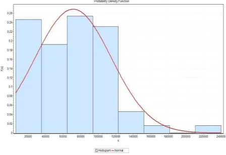
Figure 1: Histogram of Claim Amounts with a Normal Distribution curve superimposed.

From the histogram, the claims distribution is heavily skewed to the right. This is particularly a useful feature of our data. Most general insurance data are often skewed to the right. This can simply be explained as more claims of relatively small amounts occur as compared to claims with larger compensation. This skewness is also confirmed by the numerical value of 0.53931 in the descriptive statistics. Even before we perform further analysis, it can be inferred that, distributions with heavy tails will fit our data properly. Candidates are, Pareto, Weibull, Gamma, Normal.

Figure 2: Q-Q Plot of the normal distribution.

Q-Q plot is a measure of how the empirical distribution of data fits the specified model. It basically provides a visual inference as to whether the distribution specified fits the data it’s been used to model.

4.2

Time

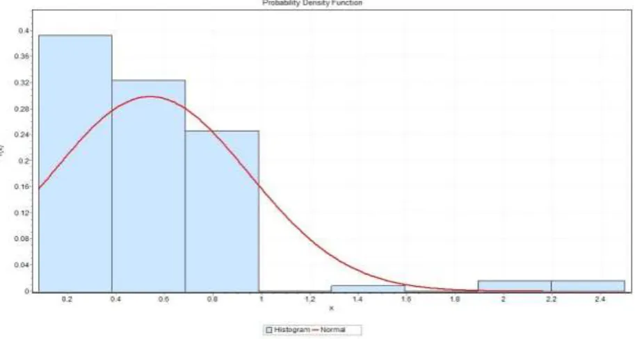
We followed the same procedure for fitting a model to the time of claim occurrence. A histogram plot is as shown below.

Based on the chi-square goodness of fit test and the Q-Q plot, the Weibull distribution was chosen as best fit for the time band.

5

Simulation Procedures

Having fitted the appropriate probability distribution to the claim amounts and the time of occurrence, in this section, we discuss the claims simulation process as a means of predicting future claim occurrence. We used simulation by inversion. The following variables are defined to aid in this process.

5.1

Variables

• Tj = time of a claim payment. • Tj = Cj + Lj.

• Cj = time of claim intimation (occurrence). • Lj = time from occurrence to payment.

Assuming the Lj’s are independent of each other.

Let the time between events Cj − Cj−1 (Co = 0) be independent and identically distributed with an exponential distribution (θ)

Let Xj be the amount paid at time Tj on a loss that occurred at Cj.

Amount Xj and Cj are independent but Xj and Lj are positively correlated. The reason been that, claims of larger amounts take a long time to settle compared to claims of small amounts.

We define Vt to be the discount factor which is independent of Xj, Cj, Lj but for s 6= t, Vs and Vt are dependent.

Thus, for an exposure, expected present value of claims is given by

N

S = XXjVTj N = maxCj < L{j}

j=i

From our distribution fitting process, the amount of a payment(Xj) have a Normal distribution with µ = 5527.3 and σ = 9123.1

The time from the occurrence of a claim to its payment(Lj) have a Weibull distribution with α = 1.5504, to model the

dependence relation, we let the scale parameter of the Weibull distribution depend on the claim size, thus

For the discount factor, we assumed that for has a Normal distribution with mean µ and variance σ2 (t − s)

5.2

Inverted Distributions

Working within a one-year time period.

• First generate exponential inter-loss times until their sum exceeds one. This gives one-year worth of claims.

If ui are the pseudo-uniform variates;

xi = θ ln(1 − ui) xi = 0.5424ln(1 − ui)

This gives Cj in incremental fashion.

• Next, we generate loss amounts corresponding to the number of inter-loss times. Loss amounts follow a Normal distribution. For ui pseudo-uniform variate

• Deriving the Ljs. Recalling that they follow a Weibull distribution; for ui pseudo-uniform variate;

1 _li = −θ (ln(1 − _u i))α

With the Lj’s in hand, the payment times can be obtained as tj = cj + lj

6

Simulated Claims

A portfolio consisting of 173 policyholders was constructed to run test the model.

A discounting factor was applied to the claim occurrence to find their present value at policy inception.

This present value is termed as the aggregate expected claim of a policyholder. A histogram was fitted to these aggregate claim records.

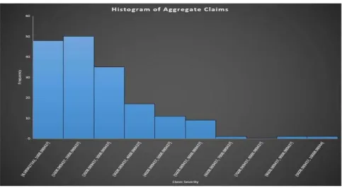
Figure 4: A Histogram of the Aggregate Claim Amounts

It can be inferred from the histogram that the portfolio is characteristic of a general insurance portfolio. The heavily skewed right distribution of the aggregate claims also supports our earlier assertions that, the generated claim records from the IRDAI fits a heavy tail distribution.

7

Pure Premium

Having obtained the claim records, we proceed to determine the individual pure premiums based on our pricing model.

The CBOE VIX was observed to be 12.75.2

The long-term was observed to be 15.39% whiles the mean returns, Ms&p500 was observed to be

8.77%.

The standard deviation of equity option price returns over a one-year period was observed to be 12.75%.3

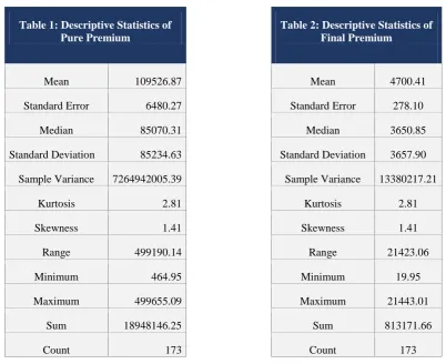
Table 1: Descriptive Statistics of Pure Premium

Table 2: Descriptive Statistics of Final Premium

Mean 109526.87 Mean 4700.41

Standard Error 6480.27 Standard Error 278.10

Median 85070.31 Median 3650.85

Standard Deviation 85234.63 Standard Deviation 3657.90

Sample Variance 7264942005.39 Sample Variance 13380217.21

Kurtosis 2.81 Kurtosis 2.81

Skewness 1.41 Skewness 1.41

Range 499190.14 Range 21423.06

Minimum 464.95 Minimum 19.95

Maximum 499655.09 Maximum 21443.01

Sum 18948146.25 Sum 813171.66

Count 173 Count 173

Computing the standardized market price of risk(It) for a one-year period, we obtain 0.07266.

With all the relevant common parameters obtained, we now computed the individual pure premiums. A scatter plot of the computed pure premiums4 is as shown in Figure 5.

Figure 5: Scatter Plot of Pure Premiums

There is no systematic trend in the premiums. This is a particularly useful feature of the portfolio. There is visibly, an outlier in the portfolio. This policyholder premium is particularly high and can be explained from two different angles.

First, there is a possibility that she has a high variation in her claim experience, leading to a relatively high coefficient of loss variation culminating in to high premium. This might probably reduce her premium when savings is taken into consideration.

Another possibility is that, she may have a stable claim experience but with a relatively high claim amount. This will particularly not change much even with the application of savings.

Summary Statistics of the pure premiums is as shown in Table 1

The average yearly pure premium for the portfolio is 109,526.87 Indian Rupee. This is a ’stand-alone’ individual premium and is quite high.

In the next section, we will see how the portfolio can contribute to reducing the premium.

7.1

Claims Portfolio

Having obtained the pure premiums, it now stands to compute the portfolio parameters. A summary of the various quantities is contained in the table below.

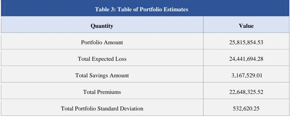
Table 3: Table of Portfolio Estimates

Quantity Value

Portfolio Amount 25,815,854.53

Total Expected Loss 24,441,694.28

Total Savings Amount 3,167,529.01

Total Premiums 22,648,325.52

Total Portfolio Standard Deviation 532,620.25

These portfolio quantities where applied to the respective formulas.

Figure 6: Histogram of Premiums with Savings

It can be inferred from the histogram (Figure 6) that, about 70% of policyholders pay relatively low premiums. Very few policyholders experience high premiums.

Interesting comparisons between the pure premiums and the premiums with savings can be inferred from the scatter plot and computed descriptive statistics.

From the scatter plot (Figure 7) and the descriptive statistics, the portfolio had a great impact on the premiums.

Note that there is a drastic reduction in the average premium from 109526.86 Indian Rupee to 4,700.41 Indian Rupee.

The Premium value obtained using the Financial model and that from the Traditional Model may now be compared. It is interesting to note that, on average, the traditional method of pricing yields Indian Rupee

4,931.00 based on statistics from IRDAI, whilst that churned out by our Financial Model amounted to Indian Rupee 4,700.41.

Given the availability of data in Ghana, and all other assumptions remaining unchanged, we are confident that this Pricing Model may be effectively applied to the Ghanaian insurance setting.

Overall, the goal of a portfolio in our model has been achieved and our research objective of developing a model that will churn out competitive premiums is a success.

8

Conclusion and Recommendations

It has been clearly demonstrated from the final results of the model generated that more efficient results in terms of cost and savings were realized, being the primary objective of this work, making insurance products priced using this model more attractive to prospective assureds.

In the course of this paper, some recommendations to be adhered to by the insurance companies, in order to obtain efficient pricing results have been identified, and these could immensely improve marketability of the insurance products. Some of these are summarized below:

It is recommended that a paradigm shift is adopted in the pricing of insurance products, as it is evident from this work that financial methods of pricing are more efficient, compared to the traditional methods of pricing insurance.

This paper did not account for life insurance products; thus, we leave it as an attractive future research area given that preliminary results from this work has proven to be promising in the case of general insurance, specifically, motor insurance.

References

[1] Wolfgang Buchholz and Michael Schymura. Expected utility theory and the tyranny of catastrophic risks. Ecological Economics, 77:234–239, 2012.

[2] Hans Bu¨hlmann. The general economic premium principle. Astin Bulletin, 14(01):13–21, 1984.

[3] Stephen P D’arcy. On becoming an actuary of the third kind. 1989.

[4] Stephen P D’Arcy and James R Garven. Property-liability insurance pricing models: an empirical evaluation. Journal of Risk and Insurance, pages 391–430, 1990.

[5] Neil A Doherty and James R Garven. Price regulation in property-liability insurance: A contingent-claims approach. The Journal of Finance, 41(5):1031–1050, 1986.

[6] Paul Embrechts. Actuarial versus financial pricing of insurance. The Journal of Risk Finance, 1(4):17–26, 2000.

[7] Jon Holtan. Pragmatic insurance option pricing. Scandinavian Actuarial Journal, 2007(1):53–70, 2007.

[8] Ravi Jagannathan and Zhenyu Wang. The conditional capm and the cross-section of expected returns. The Journal of finance, 51(1):3–53, 1996.

[9] Edi Karni. Savagesˆa subjective expected utility model. 2005.

[10] Roger JA Laeven and Marc J Goovaerts. Premium calculation and insurance pricing. Encyclopedia of Quantitative Risk Analysis and Assessment.

[11] Chris K Madsen, GE Insurance Solutions, Svend Haastrup, and Hal W Pedersen. A further examination of insurance pricing and underwriting cycles. 2005.

[12] Robert C Merton. Theory of rational option pricing. The Bell Journal of economics and management science, pages 141–183, 1973.

[13] Robert A Pollak. Additive von neumann-morgenstern utility functions. Econometrica, Journal of the Econometric Society, pages 485–494, 1967.

[14] John Quiggin. A theory of anticipated utility. Journal of Economic Behavior & Organization, 3(4): 323–343, 1982.

[15] Neeza Thandi Sholom Feldblum. Financial pricing models for property-casualty insurance products.” investment yields. The Bell Journal of economics and management science, pages 141–183, 2002.

[17] Son Van Lai and Michel Gendron. On financial guarantee insurance under stochastic interest rates. The GENEVA Papers on Risk and Insurance-Theory, 19(2):119–137, 1994.

[18] Shaun S Wang. A universal framework for pricing financial and insurance risks. Astin Bulletin, 32(02): 213– 234, 2002.

[19] Shaun S Wang. Equilibrium pricing transforms: new results using buhlmannˆas 1980 economic model. Astin Bulletin, 33(01):57–73, 2003.

[20] Shaun S Wang, Virginia R Young, and Harry H Panjer. Axiomatic characterization of insurance prices. Insurance: Mathematics and economics, 21(2):173–183, 1997.

[21] Geoff Werner and Claudine Modlin. Basic ratemaking.

[22] Menahem E Yaari. The dual theory of choice under risk. Econometrica: Journal of the Econometric Society, pages 95–115, 1987.

APPENDICES

Appendix A

Input Data Set from IRDAI

Appendix B

Python Code to Simulate the Cjs

import random import math from scipy.stats import norm import numpy as np import csv import os

def ExpTime(mean = 1.9311): #old value is 1.8437 for i in range(0, 200):

interlossSet = [] #list~immutable

ExpTimes = set(interlossSet)

#declared this way to allow for greater... #manipulations compared to an ordinary dictionary. time_Cj = [] time_Cjs = set(time_Cj)

#Above are set to null since the end output after each loop is... #written to a file and there not stored to a set to free memory count = sum(interlossSet) #loop count time_increment = 0 while(count < 1):

unif = random.uniform(0, 1)

time = -(1/mean)*math.log(1-unif) #inversion time_increment = time_increment + time

#dynamically calculate the claiam occurence period count = count + time unif_round = round(unif, 2) time_round = round(time, 2) time_increment_round = round(time_increment, 2)

time_Cj.append(time_increment) unif_time = (unif_round, time_round) interlossSet.append(unif_time)

#this generates the exponential times, compute...

#the increments by adding the current to all the previous times.

file_time = open(’C:/Python33/Projects/time.txt’, ’a’) file_cjs =

open(’C:/Python33/Projects/cjs.txt’, ’a’) interlossSet = tuple(interlossSet) #mutability transform time_Cj = tuple(time_Cj) ExpTimes.add(interlossSet) time_Cjs.add(time_Cj) writable_time = str(ExpTimes) + ’\r\n’ + ’\r\n’

#you can only write string values to a file--line break added for easy perusal writable_cjs = str(time_Cjs) + ’\r\n’ + ’\r\n’ file_time.write(writable_time) file_cjs.write(writable_cjs)

Appendix C

Python Code to Simulate the Loss Amounts

’’’

Lose Generation code

Fitted Distribution is the Normal

’’’ def Normal(number):

#Gaussian Distribution

#Discount factors will use the same function but with different mean and sigma sigma = 5527.3 mean = 9123.1

#Can convert them to inputs later

Claim = []

Claim_set = set(Claim) for i in range(number):

unif = random.uniform(0, 1) inverse_normal = norm.ppf(unif) loss = sigma*inverse_normal + mean

#seemingly buggy but ohk to avoid negative losess loss = abs(loss) Claim.append(loss)

Claim = tuple(Claim) Claim_set.add(Claim) claims =

Appendix D

Python Code to Simulate the Ljs

def Weibull(number, loss_set):

#for generating the Ljs

#Weibull Distribution shape = 1.5504

#scale = ’’ #this will depend on the loss amount to model the dependence time = [] time_set = set(time) loss_list = list(loss_set) for i in range(number): x = loss_list[i] x = float(x)

#print(x) #print(type(x)) scale = math.log(x)/7 unif = random.uniform(0, 1)

#print((1/shape))

#print(math.pow((math.log(1-unif)),1/shape )) time_unit =

scale*math.pow(abs((math.log(1-unif))), 1/shape) time.append(time_unit)

time = tuple(time) time_set.add(time) times =

open(’C:/Python33/Projects/Ljs.txt’, ’a’) writable_times = str(time_set) + ’\r\n’ + ’\r\n’ times.write(writable_times)

Appendix E

Python Code to Compute the Discount Factors

def DiscountFactors(): #Gussian Distribution

#Discount factors will use the same function but with different mean and sigma sigma = 0.39419 mean = 0.51785 variance = 0.1554

#Can convert them to inputs later

Discount = []

#Discount_set = set(Discount) timeBand = csv.reader(open("TimeBand.csv"), delimiter=",")

#csvDiscount = open(’Discount.csv’, ’w’)

#first get the simulated value

#run it through the algotithm

#change the variance on each instant in simulating the value for row in timeBand: counter = 0 value_s = 1 count=0 Discount = [] for time_value in row:

if time_value !=’’:

rand = np.random.normal(mean, sigma) denominator = float(abs(rand))*float(variance)*

(float(time_value) -float(counter)) value_t = value_s/math.exp(denominator) a = value_s b = math.exp(denominator)

#this is meant to correct discount factors exceeding one if a > b :

value_t = value_t * 0.6

Discount.append(value_t) else:

Discount.append(value_t)

#csvDiscount.writerow(’\n’)

#seemingly buggy but ohk to avoid negative times counter = row[count] count = count + 1 value_s = value_t else:

exit

with open(’Discount.csv’, ’a’, newline=’’) as csvDiscount:

#csvDiscount.writerows(value_t) wtr = csv.writer(csvDiscount, delimiter= ’,’) wtr.writerow(Discount)

csvDiscount.close

Appendix F

VBA Source Code for Evaluating the Premiums

Sub Premiums()

Dim d_1 As Double

Dim d_2 As Double

Dim r As Double

Dim D As Double

’pClaim As Double ’var As Double

Dim LastRow As Integer

Dim I_t As Double

Dim dblNorm_S_Dist As Double

I_t = 0.0726 S_t = 12.75 alpha_loss = 1.754846 r = 0.053

With ThisWorkbook.Sheets("Claims")

LastRow = .Cells(.Rows.Count, "A").End(xlUp).Row

End With

For i = 2 To LastRow Step 2

Value = ThisWorkbook.Sheets("AggregateClaims").Cells(i, 1).Value var = (ThisWorkbook.Sheets("MeanDeviation").Cells(i, 3).Value) * I_t

D = ThisWorkbook.Sheets("AggregateClaims").Cells(i, 3).Value

If var <> 0 Then

’black scholes d1 and d2 values(refer to project) d_1 = (Log(Value / D) - (0.5 * (var) ^ 2 + r)) / var d_2 = d_1 - var

Else

var = 0.5 * I_t d_1 = (Log(Value / D) - (0.5 * (var) + r)) / var d_2 = d_1 - var

’takes care of the posibility of having zero CoV End If

n_d1 = WorksheetFunction.NormSDist(-d_1) n_d2 = WorksheetFunction.NormSDist(-d_2)

’Premium = (Value * n_d1) - (D * Exp(r) * n_d2) Premium = (D * Exp(r) * n_d2) - (Value * n_d1)

ThisWorkbook.Sheets("Premiums").Cells(i, 1).Value = Premium

Next i

ThisWorkbook.Sheets("Premiums").Cells(1, 2).Value = "Savings"

ThisWorkbook.Sheets("Premiums").Cells(1, 3).Value = "Final Premium" End Sub

Appendix G

VBA Source Code for Computing the Portfolio Quantities

Sub Portfolio()

’portfolio standard deviation ’fund amount

’total savings ’allocate savings

Dim VarL_i As Double

Dim Savings_Amount As Double

Dim Portfolio_Amount As Double

Dim Total_Savings As Double

Dim LastRow As Integer

Dim Individual_premium As Double

VarL_i = ThisWorkbook.Sheets("MeanDeviation").Range("B348").Value stDevL_i = Sqr(VarL_i)

’MsgBox stDevL_i

Total_Expected_loss = ThisWorkbook.Sheets("AggregateClaims").Range("A348").Value

Portfolio_Amount = WorksheetFunction.NormSDist(0.99) * stDevL_i + Total_Expected_loss

Total_Written_premiums = ThisWorkbook.Sheets("Premiums").Range("A348").Value

’MsgBox Total_Written_premiums

Savings_Amount = Total_Written_premiums - Portfolio_Amount

’MsgBox Portfolio_Amount

With ThisWorkbook.Sheets("Claims")

LastRow = .Cells(.Rows.Count, "A").End(xlUp).Row

End With

For i = 2 To LastRow Step 2

Individual_premium = ThisWorkbook.Sheets("Premiums").Cells(i, 1).Value dev = ThisWorkbook.Sheets("MeanDeviation").Cells(i, 2).Value

’savings = (dev / stDevL_i) * Savings_Amount

savings = (Individual_premium / Total_Written_premiums) * Savings_Amount

ThisWorkbook.Sheets("Premiums").Cells(i, 2).Value = savings

ThisWorkbook.Sheets("Premiums").Cells(i, 3).Value =

(ThisWorkbook.Sheets("Premiums").Cells(i, 1).Value -

ThisWorkbook.Sheets("Premiums").Cells(i, 2).Value) Next i