Please cite this article as Koushandeh A, Chamani M, Yaghobfar A, Sadeghi AA & Baneh H. 2019. Comparison of the Accuracy of Nonlinear Models and Artificial Neural Network in the Performance Prediction of Ross 308 Broiler Chickens. Poult. Sci. J. 7(2): 151-161.
Poultry Science Journal
ISSN: 2345-6604 (Print), 2345-6566 (Online) http://psj.gau.ac.irDOI: 10.22069/psj.2019.16690.1455
Comparison of the Accuracy of Nonlinear Models and Artificial Neural Network in the
Performance Prediction of Ross 308 Broiler Chickens
Koushandeh A1, Chamani M1, Yaghobfar A2, Sadeghi AA1 & Baneh H2
1Department of Animal Science, Science and Research Branch, Islamic Azad University, Tehran, Iran 2
Animal Science Research Institute of Iran, Agricultural Research, Education and Extension Organization (AREEO), Karaj, Iran
Poultry Science Journal 2019, 7(2): 151-161
Introduction
Growth can be defined as a biological process resulting from changes in the body weight of an animal and has an economic significance in livestock breeding. Some researchers are interested in analyzing the relationship between weight and its changes over the lifespan of an animal (Eleroglu et al., 2014). Animal growth represents an event caused by complex metabolic reactions, which has led to extensive studies to describe the growth characteristics using appropriate math models (Sogut
et al., 2016). The necessity of using the parameters of the growth curve and the relationship between them and other characteristics affecting the growth of an animal is considered to be the most essential determinants of the animal's growth curve (Saghi et al., 2012). The Growth curve in different animals is a good tool for describing body weight (BW) changes, which are directly related to the age of an animal (Prestes et al., 2012), and the side effects of the choice on the growth curve parameters are accepted (Tariq et al., 2013).
The Growth curve is important in describing the production of an animal since they can be estimated by using the number of daily feed requirements for growth, especially when the food intake includes various types of food additives, with reasonable accuracy (Abbas et al., 2014). The shape of the growth curve is also affected by the composition of the diet (Mohammed, 2015). The application of such estimates by predicting the nutritional requirements of animals is important in this regard, which can lead to restrictions on the level of ad libitum access to feed for animals (Lopez et al., 2000). Some nonlinear models (NLMs) such as Brody, Von Bertalanffy, Gompertz, Logistic, and Richards used to describe animal growth affected by nutritional and environmental factors (Kum et al., 2010) and the comparison of NLMs is usually recommended for selecting the best model using different assessment criteria for species, strains and even different lines (Narinc et al., 2010). Various researchers have used NLMs to study and describe the growth curve in different poultry species, including Narinc et al. Abstract
Keywords
Broiler Growth Curve Nonlinear Model Artificial Neural Network
This study aimed to investigate and compare nonlinear growth models (NLMs) with the predicted performance of broilers using an artificial neural network (ANN). Six hundred forty broiler chicks were sexed and randomly reared in 32 separate pens as a factorial experiment with 4 treatments and 4 replicates including 20 birds per pen in a 42-day period. Treatments consisted of 2 metabolic energy levels (3000 and 3100 kcal/kg), 2 crude protein levels (22 and 24%) and two sexes. Ten birds in each pen tagged and their weekly BW records were collected individually to evaluate the accuracy of predicted BW by ANN as an alternative to nonlinear regression models (Logistic, Gompertz, Von Bertalanffy, and Brody). Based on the goodness of fit criteria and error measurement statistics, the NLMs fitted the age-weight data better than ANN. The findings indicated that the performance prediction of broiler chicks using the Gompertz model (R2 = 0.9989) was more accurate than other NLMs (R2 = 0.9628 to 0.9988) and ANN (R2 = 0.95839). Therefore, the application of the Gompertz model is suggested to predict the BW changes of Ross 308 broiler chicks over time.
Corresponding author
Mohammad Chamani
Article history
(2010) in quails, Nahashon et al. (2006) in gray pheasants, Aggrey (2002), Darmani Kuhi et al. (2003), Yang et al. (2006), Ahmadi and Mottaghitalab (2007), Norris et al. (2007) and Golian and Ahmadi (2008) in broiler chicks, Vitezica et al. (2010) in Ducks, Sengul and Kiraz (2005), Porter et al. (2010) in turkeys, and Sabbioni et al. (1999) in ostriches. The most important advantage of NLMs is the use of statistical software in the design of specific mathematical functions to estimate the growth curve and the effects of nutritional needs on it (Sengul and Kiraz, 2005).
Recently, the artificial neural network (ANN) has become commonplace in predicting animal performance in addition to mathematical models. The design and programming of ANN are like a human brain, has the ability to respond to different inputs through several layers, including millions of neurons, which ultimately leads to solving a small part of a big problem. One of the main advantages of using ANN in comparison with the classic statistical modeling is that ANN modeling can only be performed based on a dependent variable and designing various types of the variable is also possible. This fact reduces wasting time, resources, a better estimation of error and variability in data collection under different
circumstances (Ahmad, 2009). Another important advantage of ANN in estimating the nutritional requirements of broiler chickens is the need to determine the best fitting model before simulating growth data (Kaewtapee et al., 2011). On the other hand, ANN models have been introduced in many breeding systems as an alternative to regression analysis for predicting broiler chicken growth performance (Ahmad, 2009; Roush et al., 2006).
This study was carried out to evaluate and describe the performance prediction of Ross 308 broiler chicks by comparing the fitting growth data set using ANN and NLMs.
Materials and methods
Six hundred forty Ross 308 broiler chicks were sexed and reared in 32 pens with separate dipping and drinking water. Ten chicks from each pen were randomly selected and tagged. The treatments were carried out in a factorial experiment using a completely randomized design with 2 levels of metabolic energy (3,000 and 3,100 kcal/kg), 2 levels of crude protein (22 and 24%) and two sexes which were repeated 4 times. The nutritional treatments used are shown in table 1.
Table 1. Composition percentage of experimental diets in starter, grower and finisher phases
Ingredients (%) Starter (1-10 days) Grower (11-25 days) Finisher (26-42 days)
T1 T2 T3 T4 T1 T2 T3 T4 T1 T2 T3 T4
Corn 57.29 50.60 56.14 49.00 57.38 55.00 55.80 53.30 62.50 59.10 60.00 57.80
Soybean Meal (%48) 37.0 42.69 37.0 43.0 35.92 38.1 35.8 38.0 30.5 33.4 31.0 33.2
Soybean Oil 2.00 3.00 3.20 4.40 3.40 3.60 5.00 5.30 4.00 4.50 6.00 6.00
Oyster Shell 0.80 0.80 0.80 0.80 0.70 0.70 0.80 0.80 0.65 0.65 0.65 0.65
Defloured Phosphate 1.71 1.71 1.70 1.70 1.50 1.50 1.50 1.50 1.30 1.30 1.30 1.30
Salt 0.22 0.22 0.22 0.20 0.20 0.20 0.20 0.20 0.20 0.20 0.20 0.20
Vitamin Premix1 0.25 0.25 0.25 0.25 0.25 0.25 0.25 0.25 0.25 0.25 0.25 0.25
Mineral Premix2 0.25 0.25 0.25 0.25 0.25 0.25 0.25 0.25 0.25 0.25 0.25 0.25
DL-Methionine 0.27 0.27 0.22 0.20 0.20 0.20 0.20 0.20 0.20 0.20 0.20 0.20
L-Lysine HCL 0.21 0.21 0.22 0.20 0.20 0.20 0.20 0.20 0.15 0.15 0.15 0.15
Calculated composition
ME (kcal/g) 3.00 3.00 3.06 3.07 3.10 3.09 3.18 3.18 3.19 3.19 3.29 3.27 Protein (%) 22.03 24.01 21.91 23.96 21.50 22.28 21.31 22.08 19.45 20.47 19.46 20.26 Ether Extract (%) 4.23 5.11 5.40 6.46 5.62 5.78 7.17 7.42 6.30 6.74 8.23 8.20 Crude Fiber (%) 4.65 4.81 4.61 4.78 4.58 4.65 4.52 4.58 4.39 4.47 4.33 4.41 Calcium (%) 0.96 0.98 0.96 0.97 0.86 0.86 0.89 0.90 0.76 0.77 0.76 0.76 Available Phosphorus (%) 0.45 0.46 0.45 0.46 0.41 0.42 0.41 0.41 0.37 0.37 0.37 0.37 Lys (%) 1.28 1.42 1.29 1.42 1.25 1.30 1.24 1.29 1.08 1.15 1.08 1.14 Met (%) 0.58 0.60 0.53 0.53 0.50 0.51 0.50 0.51 0.48 0.49 0.48 0.49 Cys (%) 0.32 0.34 0.31 0.34 0.31 0.32 0.31 0.32 0.28 0.30 0.28 0.29 TSAA (%) 0.90 0.94 0.84 0.87 0.81 0.83 0.81 0.83 0.77 0.79 0.76 0.78 1
Provided per kg of diet: 44000 IU A, 17000 IU D3, 440 mg E, 40 mg K3, 70 mg B12, 65 mg B1, 32 mg B2, 49 mg Pantothenic acid, 122 mg Niacin, 65 mg B6, 22 mg Biotin and 27 mg Choline chloride.
2Provided per kg of diet: 99.2 mg Mn (MnO), 85 mg Zn (ZnO), 50 mg Fe (FeSO
4), 10 mg Cu (CuSO4), 0.2 mg Se (Na2SeO3), 13
mg I (KI), and 250 mg Co
The breeding broiler management and ratio formulation were both based on the catalog of Ross 308 (2016). The guide for the care and use of laboratory animals was followed, and the project was approved by
Koushandeh et al., 2019 153
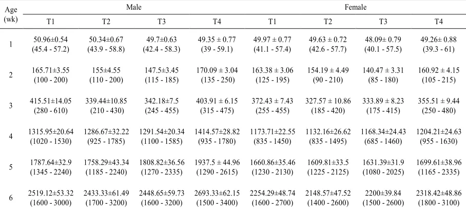
Table 2.Statistical description of recorded body weight data for two sexes (Means ± SE (Range: Min -Max))
Age (wk)
Male Female
T1 T2 T3 T4 T1 T2 T3 T4
1 50.96±0.54 (45.4 - 57.2)
50.34±0.67 (43.9 - 58.8)
49.7±0.63 (42.4 - 58.3)
49.35 ± 0.77 (39 - 59.1)
49.97 ± 0.77 (41.1 - 57.4)
49.63 ± 0.72 (42.6 - 57.7)
48.09± 0.79 (40.1 - 57.5)
49.26± 0.88 (39.3 - 61)
2 165.71±3.55 (100 - 200)
155±4.55 (110 - 200)
147.5±3.45 (115 - 185)
170.09 ± 3.04 (135 - 250)
163.38 ± 3.06 (125 - 195)
154.19 ± 4.49 (90 - 210)
140.47 ± 3.31 (85 - 180)
160.92 ± 4.15 (105 - 215)
3 415.51±14.05 (280 - 610)
339.44±10.85 (210 - 430)
342.18±7.5 (245 - 455)
403.91 ± 6.15 (315 - 475)
372.43 ± 7.43 (255 - 455)
327.57 ± 10.86 (185 - 420)
333.89 ± 8.23 (175 - 415)
355.51 ± 9.44 (250 - 480)
4 1315.95±20.64 (1020 - 1530)
1286.67±32.22 (925 - 1785)
1291.54±20.34 (1100 - 1585)
1414.57±28.82 (935 - 1780)
1173.71±22.55 (835 - 1450)
1132.16±26.62 (835 - 1495)
1168.34±24.43 (685 - 1460)
1204.21±24.63 (955 - 1630)
5 1787.64±32.9 (1345 - 2240)
1758.29±43.34 (1185 - 2240)
1808.82±36.56 (1270 - 2335)
1937.5 ± 44.96 (1290 - 2615)
1660.86±35.46 (1230 - 2130)
1609.81±33.5 (1225 - 2125)
1631.39±31.9 (1080 - 2025)
1699.61±38.96 (1165 - 2335)
6 2519.12±53.32 (1600 - 3000)
2433.33±61.49 (1700 - 3200)
2448.65±59.73 (1600 - 3200)
2693.33±62.15 (1500 - 3400)
2254.29±48.74 (1600 - 2700)
2148.57±47.52 (1400 - 2600)
2200±39.84 (1500 - 2600)
2318.42±48.86 (1800 - 3100)
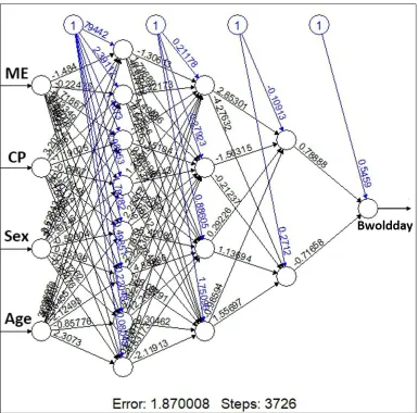
The artificial neural network (ANN) used in this research was multi-layer perceptron (MLP), composed of three connected feed-forward layers of neurons named as input, hidden and output (Rumelhart & McClelland, 1986). The input layer consisted of ME, CP, sex, and age that were connected to three hidden layers and the output layer was predicted weight. The following functions used in this type of ANN were hyperbolic tangent in the hidden layers and the active linear function in the output layer.
Hyperbolic function in hidden layers:
( ) = −
+ Active linear function in the output:
( ) =
Where, f(x) and x represent the output of the function from neurons and the weighted sum of inputs or the width of the basis function, respectively.
The ANN was designed by using the neuralnet package of the R software (2017). Age, sex, and different levels of ME and CP were considered as input layers of ANN along with three hidden layers and the predicted weight formed the output (Figure 1). Seventy-five percent of the weight record data was used as training data and other samples were used as test data for validating of the model and various states of the ANN structure including the number of neurons, intermediate layers, and learning periods were applied to describe the growth curve in broilers. To investigate the relationship between age, sex, ME and CP with BW of broilers, the NLMs including Logistic, Gompertz, Von Bertalanffy, and Brody were used to fit the growth data set by the NLIN procedure of SAS software (2013) as follows. Logistic model: = ∗ [(1 + ∗ (− )) ] Gompertz model: = ∗ exp[− ∗ (− )]
Von Bertalanffy model:
= ∗ [(1 − ∗ (− )) ]
Brody Model: = ∗ [1 − ∗ (− )]
Where, Wt represents the BW at age t and the parameters of A, B, and k, represents the maturity weight, initial weight and maturity rate, respectively. The estimated parameters (A, B and k) were analyzed by GLM procedure (SAS 2013), and Duncan’s multiple range test (α=0.05) used for means comparison between sex and treatment levels (Duncan, 1955). The accuracy of the NLMs was measured by calculating the following criteria (Kaewtapee et al., 2011; Masoudi, 2017).
1. The Pearson correlation coefficient (PCC):
ŷ = ( ,ŷ )
. ŷ (Equation 1.)
2. The coefficient of determination (R2):
= 1 − ∑ ( ŷ )
∑ ŷ ∑ ŷ
(Equation 2.)
3. The root of mean square error (RMSE):
= ∑ ( ŷ ) (Equation 3.)
4. Mean absolute deviation (MAD):
=∑ | ŷ | (Equation 4.) 5. The Mean absolute percentage error (MAPE):
=
∑ ŷ
× 100 ; ( ≠ 0)
(Equation 5.) 6. The Akaike information criterion (AIC):
= 2 − 2 = × ln + 2
Results and Discussion
All nonlinear models converged in terms of the individual weight of broiler chicks. The estimated
values of the parameters of NLMs and ANN along with the statistics of estimation for each model are presented in table 3.
Table 3. Estimated parameters of non-linear models and artificial neural network Model
parameters
Nonlinear regression models
ANN
Logistic Gompertz Von Bertalanffy Brody
A 3294.7703±819.6601 5797.182±1955.9871 15320.6709±9529.6648 9963.5049±433.3521 ―
B 40.0051 ± 11.2784 5.0009 ± 0.4595 0.8873 ± 0.0303 1.0287 ± 0.0335 ―
k 0.1137 ± 0.0178 0.0443 ± 0.0118 0.0196 ± 0.009 0.0439 ± 0.0152 ―
CV 5.20043 4.29973 4.40472 22.42431 ―
PCC 0.99816
(< 0.0001)
0.99878 (< 0.0001)
0.99872 (< 0.0001)
0.96281
(< 0.0001) 0.97962
R2 0.99837 0.99895 0.99889 0.96719 0.95959
RMSE 50.9648 40.68236 42.53597 223.84191 166.02934
MAD 37.84551 27.97285 30.8842 183.54734 102.6055
MAPE 17.26078 8.61803 10.6297 103.29908 12.96117
AIC 16528.62987 13588.03117 11928.61241 42858821.6028 29325.36
A: Asymptotic or mature weight, B: Initial weight, k: Growth rate, CV: Coefficient of variance, PCC: Pearson correlation
coefficients between predicted and actual BW, R2: Coefficient of determination, RMSE: Root of mean square error, MAD:
Mean absolute deviation, MAPE: Mean absolute percentage error, AIC: Akaike information criterion
Koushandehet al., 2019 155
The Gompertz model was superior to the Von Bertalanffy, Logistic and Brody models with regard to R2, RMSE, MAD, MAPE and PCC. However, the weakest amount of AIC belonged to the Von Bertalanffy model. The Gompertz equation comes as follows.
= 5797.182 ∗ [−5.0009 ∗ (−0.0443 )]
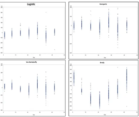
In addition, the Gompertz model was determined for RMSE as the best nonlinear model, although the lowest R2 value was unexpectedly observed in the ANN model (R2 = 0.95959). The comparison of fitting plots and residual-age diagrams indicated that estimated BW by the Gompertz model had the best overall fit (Figures 2 and 3).
The shape of growth curves in the Logistic, Gompertz and ANN models were better fitted to the observed BW data set. The estimated value for the maturity weight (parameter A) of Logistic and Gompertz models were more symmetric than other NLMs to the observed BW data set. The most predicted value of initial weight (parameter B) belonged to the Logistic model. The Von Bertalanffy model had the highest slope of the growth curve which was directly affected by the maturity rate (parameter k). The comparison of NLMs in order to select the best fitting model was determined by measuring the error of each model using various criteria such as MAD and RMSE.
Table 4. Estimated parameters of non-linear models for male and female broilers Model
parameter
Nonlinear regression models
Logistic Gompertz Von Bertalanffy Brody
Male:
A 3535.07 ± 964.5813 5914.51 ± 2025.96 16201.95 ± 9827.47 9912.21 ± 681.2076
B 42.2461 ± 13.354 5.0977 ± 0.4796 0.8954 ± 0.0328 1.0349 ± 0.0526
k 0.1154 ± 0.0209 0.0462 ± 0.0131 0.0198 ± 0.0088 0.048 ± 0.0226
PCC 0.99782 0.99873 0.99864 0.96091
R2 0.99807 0.99891 0.99882 0.96535
RMSE 58.55798 45.90971 46.79243 242.71306
MAD 43.65951 32.19886 34.45277 198.16451
MAPE 18.29051 9.21634 11.45374 109.10697
AIC 8760.53726 6653.11083 6909.3368 22257226.32124
Female:
A 3036.42 ± 611.9564 5648.97 ± 1906.11 14453.8 ± 9256.33 10000 ± 0
B 37.8253 ± 9.4693 4.9136 ± 0.4351 0.8798 ± 0.0263 1.0244 ± 0.0119
k 0.1125 ± 0.015 0.0428 ± 0.0107 0.0196 ± 0.0092 0.0401 ± 0.0066
PCC 0.99859 0.99895 0.99880 0.965
R2 0.99876 0.99911 0.99898 0.96962
RMSE 41.54597 35.31973 38.13825 202.18875
MAD 31.75383 24.16768 27.5544 168.23209
MAPE 16.18188 8.0793 9.86079 97.21382
AIC 7657.39451 6882.24382 6996.16192 20536108.1712
A: Asymptotic or mature weight, B: Initial weight, k: Growth rate, PCC: Pearson correlation coefficients between predicted
and actual BW, R2: Coefficient of determination, RMSE: Root of mean square error, MAD: Mean absolute deviation, MAPE:
Mean absolute percentage error, AIC: Akaike information criterion
The statistical results of the estimated parameters of NLMs for male and female broilers are presented in table 4. The R2, RMSE, MAD and MAPE criteria for both males and females in the Gompertz model were better than other NLMs. Therefore, the following Gompertz models were selected as the best descriptive functions for predicting of BW in male and female broilers.
= 5914.51 ∗ [−5.0977 ∗ (−0.0462 )]
(Male broilers)
= 5648.97 ∗ [−4.9136 ∗ (−0.0428 )]
(Female broilers)
The estimated value of parameters A and k in Logistic, Gompertz and Von Bertalanffy models in male chicks were higher than females, which indicate that male chicks had better growth than females
with the actual values of body weight but then by the end of the breeding period in both sexes, the predicted values were slightly higher than the actual values in Logistic, Gompertz, and ANN models. The
only observed exception was the Von Bertalanffy model which the predicted weight values were overestimated after 14 days of age.
Figure 2. The fit plot for prediction of non-linear models
Table 5. Duncan’s multiple range test for parameters of non-linear models of male and female broilers
Model parameters Nonlinear regression models
Logistic Gompertz Von Bertalanffy Brody
A
Male 3535.07a 5914.5 16202 9912.21
Female 3036.42b 5649 14454 10000
SEM 48.4553 45.2442 628.7965 227.9611
F-value (p-value)
28.59**
(< 0.0001)
1.11ns
(0.292)
2.2ns
(0.1391)
2.43ns
(0.1198) B
Male 42.246a 5.09767a 0.895358a 1.034863a
Female 37.825b 4.91359b 0.879837b 1.02443b
SEM 0.6747 0.0285 0.002 0.0022
F-value (p-value)
12.26**
(0.0005)
11.87**
(0.0007)
15.63**
(0.0001)
5.49*
(0.0198) k
Male 0.115375 0.046197a 0.019766 0.048018a
Female 0.112534 0.042818b 0.019612 0.0401b
SEM 0.001 0.0007 0.0006 0.001
F-value (p-value)
2.2ns
(0.139)
5.8*
(0.0167)
0.01ns
(0.9185)
16.5**
(< 0.0001)
SEM: Standard Error of the Mean
Koushandeh et al., 2019 157
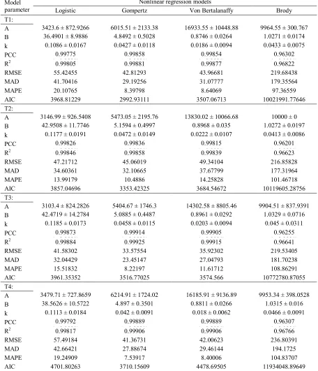
Table 6. Estimated parameters of non-linear models for different treatments of experimental diet Model
parameter
Nonlinear regression models
Logistic Gompertz Von Bertalanaffy Brody
T1:
A 3423.6 ± 872.9266 6015.51 ± 2133.38 16933.55 ± 10448.88 9964.55 ± 300.767
B 36.4901 ± 8.9886 4.8492 ± 0.5028 0.8746 ± 0.0264 1.0271 ± 0.0174
k 0.1086 ± 0.0167 0.0427 ± 0.0118 0.0186 ± 0.0094 0.0433 ± 0.0075
PCC 0.99775
(< 0.0001)
0.99858 (< 0.0001)
0.99854 (< 0.0001)
0.96302 (< 0.0001)
R2 0.99805 0.99881 0.99877 0.96822
RMSE 55.42455 42.81293 43.96681 219.68438
MAD 41.70416 29.19256 31.07777 179.35564
MAPE 20.10765 8.39798 8.64069 97.36559
AIC 3968.81229 2992.93111 3507.06713 10021991.77646
T2:
A 3146.99 ± 926.5408 5473.05 ± 2195.76 13830.02 ± 10066.68 10000 ± 0
B 42.9508 ± 11.7746 5.1594 ± 0.4997 0.8968 ± 0.035 1.0272 ± 0.0197
k 0.1177 ± 0.0191 0.0472 ± 0.0149 0.0222 ± 0.0107 0.0413 ± 0.0086
PCC 0.99826
(< 0.0001)
0.99836 (< 0.0001)
0.99815 (< 0.0001)
0.96201 (< 0.0001)
R2 0.99846 0.99858 0.99839 0.96623
RMSE 47.21712 45.06019 49.34104 216.85828
MAD 34.60361 32.10665 37.67799 177.31964
MAPE 13.99179 10.4886 14.25828 101.46718
AIC 3857.04696 3353.42325 3684.54672 10119605.28756
T3:
A 3103.4 ± 824.2826 5404.67 ± 1746.3 14302.58 ± 8805.46 9904.51 ± 837.9391
B 42.4719 ± 14.2784 5.0885 ± 0.4487 0.8961 ± 0.0292 1.0329 ± 0.0716
k 0.1185 ± 0.0173 0.0458 ± 0.0115 0.0203 ± 0.0094 0.045 ± 0.0311
PCC 0.99873
(< 0.0001)
0.99914 (< 0.0001)
0.99905 (< 0.0001)
0.96255 (< 0.0001)
R2 0.99884 0.99925 0.99915 0.96641
RMSE 41.58302 33.57554 35.92302 219.53405
MAD 32.04429 23.45147 27.04793 181.70238
MAPE 15.51832 8.22197 11.61712 108.86291
AIC 3961.35352 3516.77025 3574.566 10772780.87055
T4:
A 3479.71 ± 727.8659 6214.91 ± 1724.02 16185.91 ± 9136.89 9953.34 ± 398.0528
B 38.5626 ± 10.5722 4.897 ± 0.3501 0.8811 ± 0.0266 1.0315 ± 0.016
k 0.1113 ± 0.0184 0.042 ± 0.0091 0.018 ± 0.0062 0.0466 ± 0.0091
PCC 0.99792
(< 0.0001)
0.99889 (< 0.0001)
0.99889 (< 0.0001)
0.96307 (< 0.0001)
R2 0.99817 0.99906 0.99906 0.96766
RMSE 57.49184 41.36731 42.00623 236.80391
MAD 42.66421 27.88674 29.46144 194.1725
MAPE 19.24909 7.53917 8.40006 104.83707
AIC 4701.80263 3710.15609 4478.69505 11934048.89649
Treatments: T1 (3000 kcal/kg ME, 22% CP); T2 (3000 kcal/kg, 24% CP); T3 (3100 kcal/kg, 22% CP); T4 (3100 kcal/kg, 24% CP), A: Asymptotic or mature weight, B: Initial weight, k: Growth rate, PCC: Pearson correlation coefficients between
predicted and actual BW, R2: Coefficient of determination, RMSE: Root of mean square error, MAD: Mean absolute
deviation, MAPE: Mean absolute percentage error, AIC: Akaike information criterion
The ranking of NLMs based on PCC between observed and predicted BW of broilers indicated the superiority of the Gompertz model for male and female chicks. The statistical comparison of the fitting models to the observed BW in terms of the R2 and RMSE described the accuracy of performance
Von Bertalanffy as the best model for fitting data of Jinghai yellow chicken with reference to R2. Furthermore, the Gompertz model had been
introduced as the best fitting model by Yakuboglu and Atil (2001).
Figure 3. The residual-age diagram of non-linear models
The current conclusion was also consistent with the findings of Topal and Bolukbasi (2008), which reported the Gompertz as the best model for describing BW change over time. The result of NLM comparison in male and female broilers by Duncan’s multiple range test (DMRT) is presented in table 5. In relation to maturity weight (parameter A), a significant difference (P < 0.0001) was only found in the Logistic model, while the differences in respect of initial weight (B) for all NLMs were significant. The maturity rate (parameter k) difference was significant in both of the Gompertz and Brody models which demonstrate the growth rate of males was better than females.
The effect of different treatments on the estimation of NLMs parameters is presented in table
Koushandehet al., 2019 159
Table 7. Duncan’s multiple range test for parameters of non-linear models for different treatments of experimental diet
Model parameters Nonlinear regression models
Logistic Gompertz Von Bertalanffy Brody A
T1 3423.6a 6015.5ab 16934 9964.55
T2 3147b 5473b 16186 10000
T3 3103.4b 5404.7b 14303 9904.51
T4 3479.7a 6214.9a 13830 9953.34
SEM 48.4553 45.2442 628.7965 227.9611
F-value (p-value)
11.66** (0.0007)
7.98** (0.0051)
4.07ns (0.0549)
0.03ns (0.871) B
T1 36.49b 4.84916b 0.874592b 1.027114
T2 42.951a 5.15943a 0.896774a 1.027235
T3 42.472a 5.08846a 0.896116a 1.032873
T4 38.563b 4.89702b 0.881089b 1.031492
SEM 0.6747 0.0285 0.002 0.0022
F-value (p-value)
16.67** (< 0.0001)
21.6** (< 0.0001)
22.91** (< 0.0001)
0.05ns (0.8148) k
T1 0.10859b 0.042047b 0.018569b 0.043268
T2 0.117663a 0.047218a 0.022203a 0.041346
T3 0.1185a 0.045768ab 0.020309ab 0.044988
T4 0.111346b 0.042047b 0.018031b 0.046637
SEM 0.001 0.0007 0.0006 0.001
F-value 16.04** 8.22** 6.13* 0.67ns
Treatments: T1 (3000 kcal/kg ME, 22% CP); T2 (3000 kcal/kg, 24% CP); T3 (3100 kcal/kg, 22% CP); T4 (3100 kcal/kg, 24% CP)
SEM: Standard Error of the Mean
* The difference between two means is significant (α=0.05) ** The difference between two means is significant (α=0.01) ns: The difference between two means is not significant
According to Kaewtapee, et al. (2011), the model of ANN was superior to other models with regard to R2 and RMSE, which is consistent with Ahmad (2009) and Roush et al. (2006). However, other researchers, such as Cravener and Roush (2001) believed that
ANNs based on back-propagation will not increase the potential for forecasting of the resulting models in comparison with NLMs which is consistent with the findings of this research.
0 500 1000 1500 2000 2500 3000 3500 4000
0 7 14 21 28 35 42
B
W,
g
Days
Logistic
Actual BW for Male Predicted BW for Male
0 500 1000 1500 2000 2500 3000 3500 4000
0 7 14 21 28 35 42
B
W,
g
Days
Gompertz
Figure 4. The growth curves for male and female BW prediction of non-linear models
Conclusion
The Gompertz model was better than other NLMs among the different experimental treatments in both sexes, indicating high flexibility of model in predicting the weight of broiler Ross 308 and due to the significant difference in the values of parameter k, it is recommended to separate the diets of male and
female chicks. However, the goodness of fit was better in female than male chicks and was also slightly more favorable in the high-energy diets. Because of the significant increase in k and A parameters of the Gompertz model, it is suggested to use 24% CP with 3000 and 3100 kcal/kg ME for the grower and finisher diets.
References
Abbas AA, Yosif AA, Shukur AM & Ali FH. 2014. Effect of Genotypes, Storage Periods and Feed Additives in Broiler Breeder Diets on Embryonic and Hatching Indicators and Chicks Blood Parameters. Scientia Agriculturae, 7: 44-48. DOI: 10.15192/PSCP.SA.2014.3.1.4448
Aggrey SE. 2002. Comparison of Three Nonlinear and Spline Regression Models for Describing Chicken Growth Curves. Poultry Science, 81: 1782-1788. DOI: 10.1093/ps/81.12.1782
Ahmad, HA. 2009. Poultry Growth Modeling Using Neural Networks and Simulated Data. Journal of Applied Poultry Research, 18: 440-446. DOI: 10.3382/japr.2008-00064
Ahmadi H & Mottaghitalab M. 2007. Hyperbolastic Models as a New Powerful Tool to Describe Broiler Growth Kinetics. Poultry Science, 86: 2461-2465. DOI: 10.3382/ps.2007-00086
Cravener TL & Roush WB. 2001. Prediction of Amino Acid Profiles in Feed Ingredients: Genetic Algorithm Calibration of Artificial Neural Networks. Animal Feed Science and Technology, 90: 131-141. DOI: 10.1016/S0377-8401(01) 00219-X
Duncan, D. B. 1955. Multiple Range and Multiple F Tests. Biometrics, 11: 1-42. DOI: 10.2307/ 3001478
Darmani Kuhi H, Kebreab E, Lopez S & France J. 2003. An Evaluation of Different Growth Functions for Describing the Profile of Live Weight with Time Age in Meat and Egg Strains of
Chicken. Poultry Science, 82: 1536-1543. DOI: 10.1093/ps/82.10.1536
Eleroglu H, Yildirim A, Şekeroğlu A, Çoksöyler FN & Duman M. 2014. Comparison of Growth Curves by Growth Models in Slow Growing Chicken Genotypes Raised the Organic System. International Journal of Agriculture and Biology, 16: 529-535
Golian A & Ahmadi H. 2008. Non-linear Hyperbolastic Growth Models for Describing Growth Curve in Classical Strain of Broiler Chicken. Research Journal of Biological Sciences, 3: 1300-1304.
Kaewtapee C, Khetchaturat C & Bunchasak C. 2011. Comparison of Growth Models between Artificial Neural Networks and Nonlinear Regression Analysis in Cherry Valley Ducks. Journal of Applied Poultry Research, 20: 421-428. DOI: 10.3382/japr.2010-00223
Kum D, Karakus K & Ozdemir T. 2010. The Best Nonlinear Function for Body Weight at Early Phase of Norduz Female Lambs. Trakia Journal of Sciences, 8: 62-67.
Lopez S, France J, Gerrits WJJ, Dhanoa MS, Humphries DJ & Dijkstra, J. 2000. A Generalized Michaelis-Menten Equation for the Analysis of Growth. Journal of Animal Science, 78: 1816-1828. DOI: 10.2527/2000.7871816x
Masoudi A & Azarfar A. 2017. Comparison of Nonlinear Models Describing Growth Curves of Broiler Chickens Fed on Different Levels of Corn Bran. International Journal of Avian &
0 500 1000 1500 2000 2500 3000 3500 4000
0 7 14 21 28 35 42
B
W,
g
Days
Artificial Neural Network
Actual BW for Male Predicted BW for Male Actual BW for Female 0
500 1000 1500 2000 2500 3000 3500 4000
0 7 14 21 28 35 42
B
W,
g
Days
Von Bertalanffy
Koushandeh et al., 2019 161
Wildlife Biology, 2: 34-39, DOI: 10.15406/ ijawb.2017.02.00012
Mohammed FA. 2015. Comparison of Three Nonlinear Functions for Describing Chicken Growth Curves. Scientia Agriculturae, 9: 120-123. DOI: 10.15192/PSCP.SA.2015.9.3.120123 Nahashon SN, Aggrey SE, Adefope NA, Amenyenu
A & Wright D. 2006. Growth Characteristics of Pearl Gray Guinea Fowl as Predicted by the Richards, Gompertz, and Logistic Models. Poultry Science, 85: 359-363. DOI: 10.1093/ps/85.2.359 Narinc D, Karaman E, Ziya Firat M & Aksoy T.
2010. Comparison of Nonlinear Growth Models to Describe the Growth in Japanese Quail. Journal of Animal and Veterinary Advances, 9: 1961-1966. DOI: 10.3923/javaa.2010.1961.1966 Norris D, Ngambi JW, Benyi K, Makgahlela ML,
Shimelis HA & Nesamvuni EA. 2007. Analysis of Growth Curves of Indigenous Male Venda and Naked Neck Chickens. South African Journal of Animal Science, 37: 21-26. DOI: 10.4314/ sajas.v37i1.4021
Porter T, Kebreab E, Darmani Kuhi H, Lopez S & Strathe AB. 2010. Flexible Alternatives to the Gompertz Equation for Describing Growth with Age in Turkey Hens. Poultry Science, 89: 371-378. DOI: 10.3382/ps.2009-00141
Prestes AM, Garnero ADV, Marcondes CR, Damé MC, Janner EA & Rorato PRN. 2012. Estudo da Curva de Crescimento de Bubalinos da Raça Murrah Criados no Estado do Rio Grande do Sul. Anais do 9º Simpósio Brasileiro de Melhoramento Animal. João Pessoa: ABMA.
Roush WB, Dozier WA & Branton SL. 2006. Comparison of Gompertz and Neural Network Models of Broiler Growth. Poultry Science, 85: 794-797. DOI: 1093/ps/85.4.794
Rumelhart DE & McClelland JL. 1986. Parallel Distributed Processing: Explorations in the Microstructure of Cognition: Foundations. Vol. 1: MIT Press. Cambridge. UK.
Sabbioni A, Superchi P, Bonomi A, Summer A & Boidi G. 1999. Growth Curves of Intensively Reared Ostriches Struthio Camelus in Northern Italy. Proceedings of 50thEAAP Congress, July 2000.
Saghi DA, Aslaminejad A, Tahmoorespur M, Farhangfar H, Nassiri M, Dashab GR. 2012. Estimation of Genetic Parameters for Growth Traits in Baluchi Sheep Using Gompertz Growth
Curve Function. Indian Journal of Animal Science, 82: 889-892.
SAS (Statistical Packages for the Social Sciences). 2013. SAS/STAT® 9.4. User’s Guide. SAS Institute Inc. Cary, North Carolina.
Sengul T & Kiraz S. 2005. Non-linear Models of Growth Curves in Large White Turkeys. Journal of Veterinary and Animal Science, 29: 331-337. Sogut B, Celik S, Ayasan T & Inci H. 2016.
Analyzing Growth Curves of Turkeys Reared in Different Breeding Systems Intensive and Free-Range with Some Nonlinear Models. Brazilian Journal of Poultry Science, 18: 619-628. DOI: 10.1590/1806-9061-2016-0263
Tariq MM, Iqbal F, Eyduran E, Bajwa MA, Huma ZE & Waheed A. 2013. Comparison of Non-Linear Functions to Describe the Growth in Mengali Sheep Breed of Balochistan. Pakistani Journal of Zoology, 45: 661-665.
The R Foundation for Statistical Computing. 2017. Training of Neural Network: Package ‘neuralnet’. https://cran.r-project.org/web/packages/neuralnet/ neuralnet.pdf. Accessed on February 7. 2019. The Ross 308 Broiler: Nutrition Specification. 2014.
Aviagen Publications. http://tmea.staging. aviagen. com /assets/ Tech_Center/Ross_Broiler/ Ross-308-Broiler-Nutrition-Specs-2014r17-EN. pdf
Topal M & Bolukbasi SC. 2008. Comparison of Nonlinear Growth Curve Models in Broiler Chickens. Journal of Applied Animal Research, 34: 149-152. DOI: 10.1080/09712119.2008. 9706960
Vitezica ZG, Marie-Etancelin C, Bernadet MD, Fernandez X & Granie RC. 2010. Comparison of Nonlinear and Spline Regression Models for Describing Mule Duck Growth Curves. Poultry Science, 89: 1778-1784. DOI: 10.3382/ps.2009-00581
Yakuboglu C & Atil H. 2001. Comparison of Growth Curve Models on Broilers Growth Curves I: Parameters Estimations. Online Journal of Biological Science, 1: 680-681. DOI: 10.3923/jbs.2001.682.684