Volume 16, Number 3 (2018), 437-444
URL:https://doi.org/10.28924/2291-8639 DOI:10.28924/2291-8639-16-2018-437
THE EOQ MODEL: A DIFFERENTIAL CYCLIC SYSTEM FOR CALCULATING ECONOMIC ORDER QUANTITY
RABHA W. IBRAHIM1,∗, SAMIR B. HADID2
1Faculty of Computer Science and Information Technology, University Malaya, 50603, Malaysia
2Ajman University of Science and Technology, College of Education and Basic Sciences, UAE
∗Corresponding author: [email protected]
Abstract. The EOQ model determines the quantity that minimizes the total sum of all cost functions. We suggest a common structure for economic order quantity type non-linear differential models with costs functions with respect to time in a cyclic period. For this model, we analyze the related optimization problem and develop a relaxed method for determining a bounded interval containing the optimal cycle length. Also for a special class of transportation functions, we study these consequences and introduce algorithms to calculate the optimal size and the corresponding optimal order stage.
1. Introduction
The general economy challenged by governments in recent years has been described by almost a linear
model. For such a model, it must satisfy some kind of stability. Therefore, it would be problematic to consider
it likely that decisions occupied on the basis of past actions could cause to accurate future consequences. In
view of the uncertainty and complexity usual of this setting, the question arises of the need to seek out new
methods to deal with it. One of the most dynamic features in managing any economic units is the Economic
Order Quantity (EOQ). It might be summed up, among other features, as confirming both good customer
service and efficient production while keeping records as low as possible.
Received 2018-01-27; accepted 2018-03-14; published 2018-05-02. 2010Mathematics Subject Classification. 44A45.
Key words and phrases. differential system; economic order quantity; cost function.
c
2018 Authors retain the copyrights
of their papers, and all open access articles are distributed under the terms of the Creative Commons Attribution License.
The behavior of the cost function needs not be linear. Furthermore, to be able to cover all possible conditions,
it would be sensible to signify them as variables with respect to time, position and controller. These models
usually are driven analytically by suggesting bounded intervals containing an optimal cycle length (reorder
interval) to arrive at concave functions. This method brings a minimal value of EOQ. For the other methods
of cycle optimal lengths that evaluate the upper bound by an algorithm or by utilizing some concepts of the
convex optimization problem. The convexity concept does not change in each bounded interval. In this case
the procedure calculates the interval, such that the global minimum point resides. Another structure is that
the cost function imposes in bounded intervals. Hence, the cost function is convex in all intervals; such an
algorithm introduces a local solution in each interval (see [1]). Several generalizations and modifications can
be suggested to the EOQ model, counting backordering costs and multiple units. Moreover, the economic
order interval can be computed from the EOQ and the economic production quantity typical (which controls
the optimal production quantity) can be calculated in a similar technique. The Baumol-Tobin model, has
also been utilized to compute the money demand function, where a person’s holdings of money balances can
be realized in an approach parallel to a firm’s holdings of inventory [2]. Malakooti presented a model with
conditions that could be minimized the total cost, order quantity and Shortages [3]. A historical overview
can be found in [4]. Recently, Lagodimoset et al. introduced a discrete-time EOQ model [5]. Methods for
minimization can be found in [6].
In this paper, we introduce a new mathematical modeling for EOQ. Our method is based on the fixed point
theorems in some of compact sets. The minimization of EOQ is described by considering a geometric frame
for the total cost function during a time. Our study is related to the minimum norm solution. Examples of
linear and non-linear systems illustrated in the sequel. Some of the systems have equilibrium points, which
are given approximately. This technique allows EOQ problems to be under unfixed credit period, where the
classical models are satisfied fixed credit period.
2. Processing
The model of EOQ was established by Ford W. Harris [7] under the formula:
Q=p2AB/C, (2.1)
where Ais the annual demand quantity, B is the fixed cost per item andC is the annual holding cost per
item. In this note we suggest that (2.1) changes over time taking the formula
To minimize (2.2), we shall prepare a differential equation as follows: by squaring (2.2) and differentiating
the result, we have
d
dτQ(τ) = Q(τ)
2
A0(τ) A(τ) +
B0(τ) B(τ) −
C0(τ) C(τ)
:=Q(τ) (f1(τ) +f2(τ) +f3(τ))
:=Q(τ)F(τ, A, B, C).
(2.3)
Eq. (2.3) is a general case of the suggested model (differential EOQ) given in [8]. Our aim is to find a
minimum solution for (2.3). For this purpose, we introduce the following operator Π : C → C, where C
is any closed bounded and convex subset of a Banach space B. The map Π is called non-expensive if the
following inequality holds:
kΠξ−Πηk<kξ−ηk;
and it is called a contraction mapping if
kΠξ−Πηk ≤`kξ−ηk, `∈(0,1).
We need the following outcomes:
Lemma 2.1. ( Leray-Schauder theorem) LetΠbe a continuous and compact mapping of a Banach space B
into itself, such that the set
{ξ∈B:ξ=λΠξ for some0≤λ≤1}
is bounded. ThenΠ has a fixed point.
Lemma 2.2. (Zorn’s Lemma) For any weakly compact convex subset C and any non-expansive map Π :
C→C, C has a minimal (Π-invariant) subset.
Lemma 2.3. [9] Let B be a strictly convex normed space with norm k.k. The set of fixed points of a
non-expansive mapping Π :B→Bis either empty or closed and convex.
3. Results
In this section, we introduce two cases of the functionF in (2.3).
Let the functionF, Qbe continuous with respect toτ∈J : [0, T] andF be Lipschitz with respect to (A, B, C)
kF(τ, A, B, C)−F(τ, a, b, c)k ≤℘(kA−ak+kB−bk+kC−ck).
Moreover, we letF(τ,0,0,0) = 0.Define the following operator:
(Π)(Q)(τ) := Z τ
0
Q(ς)F(ς, A, B, C)dς, Q(0) = 0.
In our study, we involve some type of specification of how EOQ moves from step to step; that isQ(τ+ 1) =
ΠQ(τ). The stationary step can be defined as a case for which ΠQ(τ) =Q(τ). This can be viewed as an
equilibrium point of the system. That is the fixed points of Π are the states at which the process of EOQ is
clear (stable).
We have the following result:
Theorem 3.1. Consider the Eq (2.3). If
℘T(kAk+kBk+kCk)≥1;
then it admits at least one solution. If
℘T(kAk+kBk+kCk)<1
then it admits a unique solution which minimizes the problem (2.2).
Proof. Obviously,
|(Π)(Q)(τ)|=|
Z τ 0
Q(ς)F(ς, A, B, C)dς|
≤
Z τ 0
|Q(ς)||F(ς, A, B, C)|dς
= Z τ
0
|Q(ς)||F(ς, A, B, C)−F(τ,0,0,0)|dς
≤℘T(kAk+kBk+kCk)kQk;
consequently, we obtain
1
℘T(kAk+kBk+kCk)|(Π)(Q)(τ)|:=λ|(Π)(Q)(τ)| ≤ kQk.
By taking the maximum value, we get
The operator Π is continuous, bounded and compact in a subset of Banach space B. Hence, in view of
Lemma2.1, the (2.3) has a solution. LetP ∈Bsuch that
(Π)(P)(τ) = Z τ
0
P(ς)F(ς, A, B, C)dς, P(0) = 0.
A calculation implies that
|(Π)(Q)(τ)−(Π)(P)(τ)|=
Z τ 0
Q(ς)F(ς, A, B, C)dς−
Z τ 0
P(ς)F(ς, A, B, C)dς
≤
Z τ 0
|Q(ς)−P(ς)||F(ς, A, B, C)|dς
≤T|F(ς, A, B, C)−F(ς,0,0,0)|kQ−Pk
≤℘T(kAk+kBk+kCk)kQ−Pk;
If ℘T(kAk+kBk+kCk) < 1 then by Banach fixed point theorem, we conclude that (2.3) has a unique
solution. It is clear that
k(Π)(Q)−(Π)(P)k ≤ kQ−Pk.
Thus operator Π is not-expensive map. Therefore, in view of Lemma2.2 and Lemma 2.3, the set of fixed
point is a minimal close convex set. Note that the fixed point corresponds to equilibrium of EOQ.
4. Examples
In this section, we shall consider some applications.
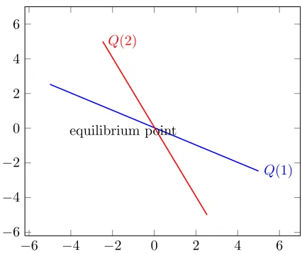
Example 1. Assume that a company’ s production in two seasons during a year satisfying the following EOQ
system:
Q(1) =A(1)B(1)−C(1)Q(2)
Q(2) =A(2)B(2)−C(2)Q(1).
(4.1)
Define the company’ s reaction functionρ:R2
+→R2+ by
If max{C(1), C(2)}<1 then a computation with respect to city block metric, gives
|ρ(Q)−ρ(Q0)|=
A(1)B(1)−C(1)Q(2)− A(1)B(1)−C(1)Q 0(2)
+
A(2)B(2)−C(2)Q(1)− A(2)B(2)−C(2)Q 0(1)
=C(1)|Q0(2)−Q(2)|+C(2)|Q0(1)−Q(1)|
≤max{C(1), C(2)}|Q0(2)−Q(2)|+|Q0(1)−Q(1)|
= max{C(1), C(2)}|Q−Q0|.
Thus, the existence and uniqueness outcome for the equilibrium, where ρ has a unique fixed point Q∗ if
C(i)<1, i= 1,2.We have the following facts:
• The conditionC(i)<1, i= 1,2 is sufficient for equilibrium but not necessary.
• This condition implies the convexity of the set of the fixed point ( Lemma2.3).
• We may replace the metric with the Euclidean metric to obtain the same result.
• In view of the conditionC(i)<1, i= 1,2 the system (4.1) can be considered as a fuzzy system (see
Fig. 1).
−6 −4 −2 0 2 4 6
−6
−4
−2 0 2 4 6
Q(1) Q(2)
equilibrium point
Figure 1: Example 1; the functions Q(1) in the horizontal axis and Q(2) in the vertical axis. Here, we
supposeC(i) = 0.5, i= 1,2.andA(i) = 0.1, B(i) = 0.3.
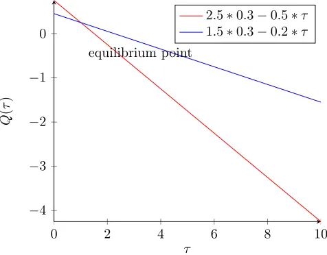
Example 2. Assume that a recent state of market isQ(0) = (Q1(0), Q2(0)).A companyj is imposingQj(0)
units. At timeτ = 1 each company selects its outcome levelQj(1) by replaying to the quantity. Consequently,
we have the system (see Fig.2)
Q1(τ+ 1) =A(1)B(1)−C(1)Q2(τ)
Q2(τ+ 1) =A(2)B(2)−C(2)Q1(τ).
The sequence< Q(τ)>converges the equilibrium pointQ∗whenever max{C(1), C(2)}<1.
0 2 4 6 8 10
−4
−3
−2
−1 0
equilibrium point
τ
Q
(
τ
)
2.5∗0.3−0.5∗τ 1.5∗0.3−0.2∗τ
Figure 2: Example 2; the functionsQ(τ) with respect toτ. We supposeC(1) = 0.5, C(2) = 0.2.
Example 3. Suppose the following non-linear system
Q1(τ) =
1 2(1 +Q2(τ))
Q2(τ) =
exp(−Q1(τ))
2 .
(4.3)
It is clear that the function%:R2
+→R2+, where
%(Q1, Q2) =
1 2(1 +Q2(τ))
,exp(−Q1(τ)) 2
is a contraction , so an equilibrium point exists and unique.
0 2 4 6 8 10
0 0.1 0.2 0.3 0.4 0.5
equilibrium point
τ
Q
(
τ
)
Q1 Q2
Figure 3: Example 3: the functions Q(τ) with respect to τ. There is a unique equilibrium point for the
Example 4. Suppose the following non-linear equationQ:R+→R+
Q(τ) =1 2
τ+C1 τ
, τ 6= 0. (4.4)
It is clear that limτ−→0Q(τ) = ∞. To minimize (2.2), we shall use the an approximation technique. The
approximation form of (4.4) is as follows:
τm+1= 1 2
τm+C 1 τm
. (4.5)
It is clear that this sequence converges to√C.Therefore, sinceQ(τ) is continuous, then√Cis a fixed point
of Q. Also, in view of Theorem 3.1, for 0<√C <1, Eq. (4.4) has a unique fixed point corresponding to
the solution of it. The reaction of (4.5) showed that it has a limit and this limit converges to the fixed point
of (4.4). Therefore, no need to show that the functionQis a contraction mapping.
5. Discussion
In general, economic can be performed by a set of fixed points; thus fixed point theorems can provide the
equilibria of economic. The frame of this work was to consider a new formula of EOQ Model. We introduced
a technique of minimizing it by using the concept of fixed point theory. We developed this method to be
suitable to the model (see Theorem 3.1). Applications are given including linear and non-linear systems.
These systems are based on changing the solution during time in a fixed interval. The equilibrium points of
each system was established, where it represented to the stationary state at which the markets clear. Also,
this stationary state acted when the company wants to change its strategy.
References
[1] R. W. Grubbstrom, Modelling production opportunities an historical overview, Int. J. Product. Econ. 41 (1995), 1-14. [2] A Caplin, J. Leahy, John, Economic Theory and the World of Practice: A Celebration of the (S, s) Model, J. Econ. Persp.
24 (1)(2010), 183-201.
[3] B. Malakooti, Operations and Production Systems with Multiple Objectives (2013). John Wiley & Sons.
[4] M.Holmbom, A. Segerstedt, Economic Order Quantities in production: From Harris to Economic Lot Scheduling Problems, Int. J. Product. Econ. 155 (2014) , 82-90.
[5] A. G. Lagodimos, et al., The discrete-time EOQ model: Solution and implications, Eur. J. Oper. Res. 266 (2018) ,112-121. [6] R. W. Ibrahim, Maximize minimum utility function of fractional cloud computing system based on search algorithm
utilizing the Mittag-Leffler sum, Int. J. Anal. Appl. 16(1) (2018), 125-136. [7] R. W. Harris, How Many Parts to Make at Once, Operat. Res. 38 (6)(1990), 947.
[8] G. Mahata, P Mahata, Analysis of a fuzzy economic order quantity model for deteriorating items under retailer partial trade credit financing in a supply chain, Math. Comput. Model. 53 (2011), 1621-1636.