Space D*

DOI 10.1007/s13173-012-0071-9 O R I G I N A L PA P E R

Space D*

A path-planning algorithm for multiple robots in unknown environments

Luan Silveira·Renan Q. Maffei·Silvia S.C. Botelho· Paulo L. Drews Jr.·Alessandro de L. Bicho·

Nelson L. Duarte Filho

Received: 10 October 2011 / Accepted: 16 March 2012 / Published online: 6 April 2012 © The Brazilian Computer Society 2012

Abstract This paper describes a new method of path-planning for multiple robots in unknown environments. The method, called Space D*, is based on two algorithms: the D*, which is an incremental graph search algorithm, and the Space Colonization algorithm, previously used to simu-late crowd behaviors. The path-planning is achieved through the exchange of information between the robots. So decen-tralized, each robot performs its path-planning, which pro-vides an obstacle-free path with the least number of robots around. The major contribution of the proposed method is that it generates paths in spacious environments facilitating the control of robots and thus presenting itself in a viable way for using in areas populated with multiple robots. The results obtained validate the approach and show the advan-tages in comparison with using only the D* method.

Keywords Path-planning·Multi-robot systems·Collision avoidance·Space Colonization algorithm·D* Lite algorithm

1 Introduction

Planning collision-free motions for autonomous robots lo-cated in environments with obstacles is one of the main problems of robotics [9,15,16].

This is a revised and extended version of a paper that appeared at ENIA 2011 (VIII Encontro Nacional de Inteligência Artificial) and has been recommended to JBCS.

L. Silveira (

Centro de Ciências Computacionais—C3, Universidade Federal do Rio Grande—FURG, Rio Grande, RS, Brazil

e-mail:[email protected]

One widely studied area of path-planning is planning in environments with multiple independent robots. For this type of problems, two approaches can be made, centralized and decoupled. In the centralized approach, planning is done by considering a single large robot made up of several seg-ments (every robot’s body), located within a large configura-tion space (corresponding to the union of the configuraconfigura-tion spaces of the robots) where each segment has a desired fi-nal configuration (the goal of each robot) [2,23]. The prob-lem with this approach is that the composed configuration space grows exponentially with the increase in robots’ num-ber, which becomes highly infeasible.

In contrast, the decoupled approach, though incomplete, reduces the problem to produce a plan for each individual robot and then adjust them [12,17]. Furthermore, viable al-ternatives are distributed decoupled techniques, which take in account the usability of distributed processing techniques to implement such approaches. In these techniques, each robot plans its path based on local knowledge and in inter-actions with other robots. The main difference between dis-tributed approaches and only-decoupled techniques is that the step of adjusting the path must be distributed and done in real time. Distributed techniques are more robust, be-cause they better accept the fails and uncertainties in the individual robots performances; in other words, a single defective robot does not interrupt the functioning of the whole.

One of the most popular algorithms that handle this type of problems is the D* algorithm (Focused Dynamic A*) [27], which adapts the optimality of A* for dynamical envi-ronments, mixing incremental searches with heuristics and achieving significant gains over repeated executions of A*.

Several works have been proposed based on D*. For ex-ample, D* Lite [14] implements the same strategy of D*, but in a simplified manner and with an efficiency equal to or greater than the efficiency of D*. In [8], it was proposed an extension to the D* and D* Lite, using linear interpolation to produce smoother paths, bypassing the issue of limited possibilities of transition between cells. Another extension of the D* Lite was proposed in [18], where the algorithm was adapted for systems with limited time. In this case, as in [29], the planning is done incrementally and further re-fined in the available time.

Another important issue is the existence of an environ-ment populated by dynamic eleenviron-ments, e.g., fleets of mobile robots. The possibility of collision between robots increases as the number of robots grows. Planning algorithms can take into account these risks in advance, leading to plans to pre-vent collisions by searching for areas with lower density of occupation.

The current work proposes an extension of the D* al-gorithm for multi-robot environments, aiming to provide a collaborative path-planning approach for multi-robot world populated. The algorithm, called Space D*, combines the D* algorithm with the Space Colonization algorithm, origi-nally designed to simulate the plant modeling [26] and later adapted for the simulation of crowd behaviors [1]. The main feature of the Space Colonization algorithm is the prefer-ence shift by spaces, to avoid the collision risk given the un-certainty and scalability of mobile and fixed obstacles. The present work is an extension of the work previously pub-lished in conference proceedings [19], where the method is better explored, and new results using real robots are showed.

In crowded environments, the difficulty of having a reli-able measure of the proximity between the robot and obsta-cles must be addressed. Methods that simply seek the short-est path tend to get closer to obstacles, requiring precise con-trol of the trajectory, for example, by reducing the speed of the robots and therefore increasing the total execution time (in spite of obtaining a lower total distance traveled). More-over, some methods that prefer free environments, such as potential fields, do not guarantee find the paths (fall into lo-cal minimal), unlike the Space D*, which inherits this char-acteristic from D*. Our approach is suitable for use in real environments by focusing on the creation of paths through environments with more free space.

This article is organized in five sections. Section 2 presents some related works about path-planning of multi-robot in unknown environments. In Sect.3, we show

tech-niques that serve as the basis for the developed method. Sec-tion4presents the path-planning algorithm proposed in this paper, dubbed Space D*. Section5provides the tests per-formed on the developed system, as well as the validation of the method. Finally, Sect.6presents the conclusions and suggestions for future work.

2 Related works

Many studies on path-planning of multiple robots are based on environments that must be completely known [7, 28]. Thus, the application of techniques such as prioritized mo-tion planning and fixed-path coordinamo-tion in unknown en-vironments can be achieved, as long as together with some approach to treatment of uncertainty.

Moreover, the algorithms for path-planning in unknown environments, such as [8,14,27], are designed to indepen-dents robots. However, they can be applied to problems with multiple robots, considering the other robots in the scenario as dynamic obstacles.

There are some works that exploit the presence of multi-ple robots with the ability to communicate and develop tech-niques for collaborative path-planning dealing with uncer-tainty. Most of the works of collaborative path-planning for multiple robots located in unknown environments focused on the problem of exploration of the environment.

In [25], the environment is separated into stripes that are explored by teams of robots and, within each team, only one robot moves at a time, reducing odometry errors. In [20], robots explore the environment randomly and exchange in-formation about obstacles when they meet. In [32], robots seek for the nearest unknown areas according to their incre-mental maps. Although, there is not coordination to prevent that two robots do the same path (improvement proposed in [3]). Later, in [4], an algorithm was proposed based on cost and utility functions to arrive at a particular uncharted location. A collaborative exploration is the focus of works like in [10] and [31], among others.

Nevertheless, there are some works focused on the path-planning itself. In [24], using navigation functions, the robots remain close to each other in order to exchange infor-mation, while they move toward their goals. In [5], robots are guided to a common destination by a specific robot, while the others are responsible for collecting the informa-tion from the environment.

Our work seeks to take in account the preference for nav-igation in nonpopulated spaces (appropriated for dynamic unknown environments), ensuring a solution path (if there is) and a collaborative mapping.

3 Underlying foundations

As mentioned earlier, the Space D* is based on two algo-rithms that are discussed briefly below: the first is the D*, widely used for path-planning in unknown environments, and the Space Colonization algorithm, which was developed for modeling plant growth [26] and used for the simulation of crowd behaviors [1].

3.1 D* algorithm

As presented, the D* algorithm [27] (replaced now by D* Lite [14]) is one of the most used and efficient approaches to the problem of path-planning in unknown environments. In fact, after its publication, the D* Lite became used in place of D* for most works, including the present work.

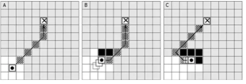
The basic behavior of the algorithm consists in recalcu-lating the shortest path to the destination whenever the cost of some cell varies (an obstacle or free space is found). This can be seen in Fig.1, where the robot’s current position is the node marked with a spot, the destination is the node marked with an “x”, and the computed path is the hatched nodes. The nodes in black and white are those with the costs al-ready observed, representing, respectively, free spaces and obstacles.

The operation of D* Lite is inspired by the A*, calculat-ing, for each node s of the graph (indicating a position on the environment), the distance to reach the goal (sgoal), and whenever the costc(s, s)to go fromsto a neighbor nodes changes (for example, if an obstacle is detected), an update of the distances of nodes affected by this change should be made.

The algorithm uses two estimates of the distance to the goal starting from a nodes, calledg(s)andrhs(s).The es-timaterhs(s)is potentially more accurate thang(s), once it

Fig. 1 Operation of D*/D* Lite. (a) The robot starts calculating a shortest path from their position (spot) to the goal (cross). (b) While moving toward the goal, it senses the environment and detect obstacles. In the case of blocked paths, a new path need to be calculated. (c) This process repeats until the goal is reached

is based on the values ofg(s)of the successors nodes ofs. The basic principle of the algorithm is keeping the two val-ues consistent for all nodes, which means that all estimates of distances are correct.

When there is any inconsistency between a pair of esti-mates, derived from the change in the cost of a node, the algorithm must update the estimates of every node affected by this change. However, to avoid going through all nodes in the graph, the D* Lite uses a heuristic to create keys that in-dicate the priority of analysis of each node. With this heuris-tic, the algorithm computes only the nodes that seem rele-vant to find the shortest path.

3.2 Space colonization algorithm

Based on studies of biology that attributed the development of veins in leaves to a hormone called auxin found in plants, the Space Colonization algorithm was developed in [26], to simulate the growth of the venation pattern in relation to the distribution of auxins in the leaves.

The algorithm is basically composed of three processes. The first is the growth of the leaf. Alongside, the other two happen: the development of the venation pattern, which is directly influenced by the distribution of the sources of aux-ins in the leaf (representing free spaces), and the generation of new auxins, which in turn is affected by the development of veins.

The vein growth begins by associating each node of auxin to the nearest vein node. Then, the nodes are expanded in the direction of the associated auxins. As the pattern grows and approaches the auxins, these are being removed, since the space that they represent is no longer free. The leaf blade grows, and new auxins are randomly generated, uniformly distributed through free space. The cycle begins again with the auxins–nodes association and continues until the leaf reaches its maximum size. As can be seen, the algorithm is characterized as a competition of vein nodes for auxins, representatives of free spaces, since the more auxins a node can be associated, the more space it has to expand.

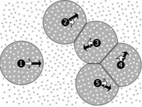
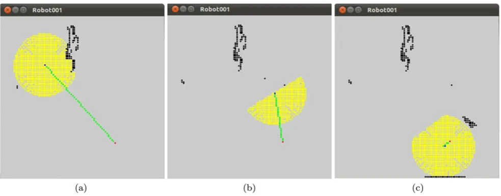
In [1], the Space Colonization algorithm was adapted to simulate crowd behaviors. The concepts of vein nodes and auxins were transformed into agents and markers of free spaces. In such a case, the Space Colonization algorithm was used to simulate the competition of agents for free space on environment.

Fig. 2 Space Colonization algorithm for simulation of crowd behav-iors.White arrowsindicate the intention of movement. Based on the free space that the agent could allocate (hatched areas), a new direc-tion of movement is calculated (black arrows)

of reaching a specific destination, not only by large availabil-ity of markers. The last one is that the speed of movement of the agents varies according the free space (in the original algorithm, the speed was uniform).

Figure2 shows an example of the algorithm execution. The agents are numbered by black circles with white arrows indicating the directions of their goals. Larger areas are the regions of markers that each agent was able to allocate. As can be observed, the restrictions in the allocated areas di-rectly influence the movement vector of each agent, repre-sented by the black arrow. Each agent seeks to move toward its goal, but avoiding the proximity to other agents or ob-stacles. The Space Colonization algorithm by itself does not solve neither the problem of path-planning in environments with obstacles nor the local minimum issues, but its feature of search for free spaces has motivated merging it with the D* Lite.

4 Space D*

The algorithm developed in this work for path-planning of multiple robots in unknown environments, named Space D*, relates the D* algorithm with the Space Colonization al-gorithm. The configuration space is represented by a grid formed by markers allocated by the nearest owner robots during the path-planning. Markers have costs which de-scribe the levels of difficulty that the robots have to reach their goals through this intersection. The owners of all mark-ers and the cost associated to them change over time. The operation of the method is, briefly, the following (for each robot):

– The environment is represented by a grid of markers that indicates the costs for a robot to cross it and to reach a goal (obstacles have the highest costs). First, the map is empty (zero cost), and as new obstacles are detected, the map is updated;

– The D* Lite algorithm is applied by each robot on the re-spective set of markers, updating the costs of these mark-ers (distances to their goals);

– The robot navigation is done using a modification upon the Space Colonization algorithm. The robot allocates all near markers, within its reach, that indicate free-spaces. With the distances to the goals of these markers, calcu-lated by the D* Algorithm, it calculates their directions of movement, which will always be defined within the allo-cated zone;

– When the robots meet each other, the information about their maps are exchanged, allowing them to update the costs of markers. In addition, the algorithm tries to avoid collisions between them, since each robot only allocates the markers that are closer to it than to other robots;

A major contribution of the proposed method is the inclu-sion in D* of the preference for navigating in less populated environments, which improves the handling of unknown and dynamic environments. In its original definition, D* gener-ates paths that tend to be very close to obstacles in order to reduce the total distance traveled, but this ends up requiring a very precise control over the movement of robots.

Another advantage of the proposed method is the ex-change of information between the robots, the focus of re-lated works, such as [13]. Since each robot obtained the map of the environment where it traveled (to perform the calcula-tion of the distance to the goal), informacalcula-tion about the pres-ence of obstacles can be exchanged when robots cross each other. This raises the possibility of avoiding paths that are blocked and that only eventually the robot would notice.

4.1 Operation of space D*

The Algorithm1shows the operation of Space D*.

Algorithm 1: Space-D* begin

whileDid not reached the goaldo Maps the environment. ifDetect other robotsthen

Exchange information. end if

Update markers cost. Run D* Lite.

Allocates the nearest markers. Calculates the direction of movement. end while

end

each position. As for the detection of robots, it was defined that each robot has a unique identifier, so that when a robot moves close enough to another, it can realize that the obsta-cle is actually a robot and also which robot.

The third stage is the exchange of information, which fol-lows the detection of robots. When two or more robots meet, both stop for a moment and exchange information corre-sponding to their descriptions of the map. It is worth noting that in the current implementation, all obstacles are static (except for the robots themselves), so the upgrade of the markers’ costs from the exchange of information consists of verifying if, in the received map, there are new obstacles that in the current map have not been discovered yet.

The fourth stage is the update of the markers’ costs, re-sulting from the steps of environment mapping and informa-tion exchange. Later, the distances to the goal starting from each marker of interest of the robot (theg(s)estimative from the D* algorithm) are computed. The processing performed in this step is, in fact, calculating the shortest path according to the D* Lite.

In the sixth stage, all markers contained in the environ-ment are associated to their nearest robot, provided that they are within the reach of the robot. The difference from the simulation of crowd behaviors [1] is that, in the proposed method, this step is decentralized, as it is up to each robot to allocate all the markers located within its reach, considering only those that are closer to themselves than to other robots. A restriction lies on the size of the radius of the allocated region. To avoid collisions between robots, it is necessary that the reach of robot perception sensor always be greater than the radius of the area of allocated markers. Ideally, the sensor reach has to be at least twice the radius of allocation, as this ensures that, in the exact moment when two robots meet, both allocate only the markers closest to them.

In the final step, to calculate its direction of motion, each robot uses the distances to the goal of the markers from their area of interest. The calculation of the movement vector−→m is a weighted vector sum of the vectors connecting the robot (−→r position) to each associated marker (−→s position):

− →_m=N

k=1

fk(−→sk− −→r ), (1)

whereNis the number of markers in the setS(r). But unlike [1], where the size of each vector was related to the direction of the goal, now the modules of the vectors are based on the distance between the marker and goal, so as the smaller the distance, the greater must be the module of a vector. The definition of the functionf that determines the magnitude of the vector of a markersassociated with the robotris f (s)= max

p∈S(r)

g(p)−g(s). (2)

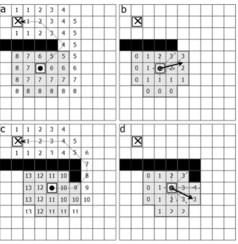
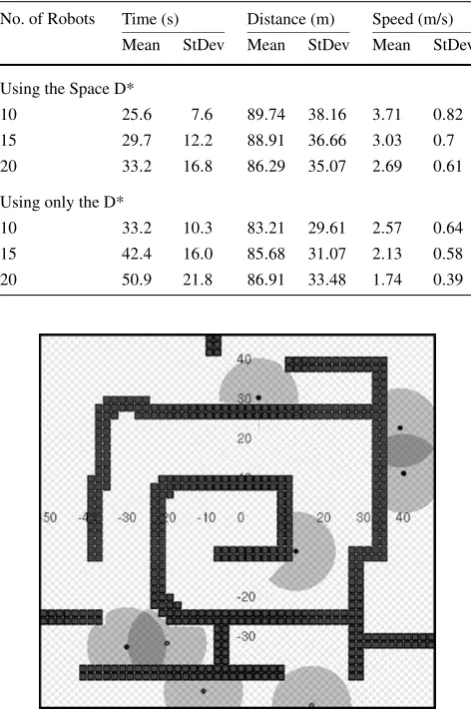
Fig. 3 Example of operation using Space D*. (a) The current map of the robot, showing the obstacles inblackand the shortest path from the current position (circle) to the goal position (cross), obtained by the execution of the D* algorithm. (b) The markers’ allocation area of the robot and the direction of movement (black arrow), obtained after the execution of Space Colonization Algorithm. (c) New obstacles are discovered in the environment, implicating update in the path to the goal. (d) The new direction of movement, based on the new allocation area and shortest path

That is, the size of each vector is the subtraction from the largest distanceg(p)of a marker belonging to the setS(r) of the robot by the value ofgof each marker.

In Fig.3, an example of the execution of the Space D* can be seen. The position of the robot is the node indicated with a spot, the goal is the node indicated with an “x”, and the obstacles are the black nodes. In (a), the demarcated area represents the allocated region of the robot, with the distances to the goal of each marker (in dotted lines is the shortest path calculated by D* Lite). In (b), the vectors are generated in the direction of the markers with the module calculated byf (s), and later, with them the movement vec-tor (larger vecvec-tor) is obtained. In (c), after moving in the direction indicated previously, the robot perceives new ob-stacles and recalculates the distances to the goal. In (d), a new movement vector is generated.

5 Tests and validation

was validated in simulated environments for multi-robots on the software Player/Stage [11], as well as using real robots controlled using Player software. A detailed de-scription of experimental results is showed in next sec-tions.

5.1 Simulated tests

The validation using simulated robots was performed by comparing the solutions obtained in the execution of the Space D* with the results of the execution of D* Lite. The simulations use omnidirectional robots with 50 cm of radius in one 100 m×100 m environment.

Spacious paths It was observed that, like the D* Lite, the Space D* generates trajectories that always reach the goal without the occurrence of collisions with obstacles, but in addition, as was predicted, it tries to maintain the robot far from any obstacle, either dynamic (other robots) or static (walls).

For the method used for comparison, the direction of movement of robots is that indicated by the shortest path computed by D*. As can be inferred, if there are no er-rors and inaccuracies in the control of robots, this tech-nique works perfectly. Yet, collisions often occur when paths are generated too close to obstacles, unless the dis-placement speeds of the robots are reduced in these loca-tions.

Figure 4 shows a comparison between the trajectories generated by the execution of the Space D* and D* on the environment showed in Fig.5. It displays the paths traveled by three robots dispersed randomly. It is possible to see that the trajectories obtained with the Space D* deviate more from obstacles than those obtained by D*, which decreases the need for speed reductions.

Average performance: execution time, distance, and veloc-ity In Table1, we compare the average execution times, average total distances, and average speeds of robots be-tween the simulations using the Space D* and the simula-tions using only the D*. In all test cases, the environment was 100×100 meters (with a discretization of 100×100 markers), and the maximum speed of robots was 5 m/s. Three test sets were evaluated (10, 15, and 20 robots), each with five random configurations of initial and final positions for each robot.

It must be repeated that in terms of the execution time of an algorithm, the Space D* makes a larger processing and thus is slower than the D* Lite. In fact, using the D* Lite, each simulation cycle was approximately half the cy-cle time of the Space D*. However, by avoiding the ap-proaching with obstacles, the Space D* allows a smaller refresh rate. In the result obtained with the Space D*, the

Fig. 4 Comparison between the trajectories was generated by the ex-ecution of the Space D* and D* for three robots. Theblack segments

are obstacles, and thegrayare the trajectories generated by the algo-rithms. We can observe on the top images that the paths generated by the D* almost touch the obstacles, which makes difficult the control of the robots. In contrast, the Space D* generates loose paths that keep the robot far from obstacles

Fig. 5 Map used to compare the D* Lite and the Space D*

average time simulation was always lower (about 30 %), be-cause although the D* obtains smaller trajectories (as can be seen by the average distance), its average speed is con-siderably lower, once the speeds of the robots are reduced in the proximity of obstacles. This indicates that the use of Space D* is more advisable, since yet the D* needs to treat the uncertainty over the configuration space and the control of robots (for instance, reducing the speed of the robots).

differ-Table 1 Comparison between Space D* and D*

No. of Robots Time (s) Distance (m) Speed (m/s) Mean StDev Mean StDev Mean StDev Using the Space D*

10 25.6 7.6 89.74 38.16 3.71 0.82

15 29.7 12.2 88.91 36.66 3.03 0.7

20 33.2 16.8 86.29 35.07 2.69 0.61

Using only the D*

10 33.2 10.3 83.21 29.61 2.57 0.64

15 42.4 16.0 85.68 31.07 2.13 0.58

20 50.9 21.8 86.91 33.48 1.74 0.39

Fig. 6 Second map used in tests

ent maps, as shown in Fig.5(the map used for the previous tests) and Fig.6with three test sets (10, 15, and 20 robots), each one with five random configurations of initial and fi-nal positions for each robot. The results are shown in

Ta-ble2. For the first map, the exchange of information did not

contributed to an improvement in execution time. Instead, it was proved worse than the method without exchange of information for a sample with 10 robots. Nevertheless, in tests with 20 robots, the method with the exchange of infor-mation was a little better. However, for the second map, the method with the exchange of information proved to be far more efficient than the method where there is no exchange of information.

It can be inferred that when obstacles are sparse and easily circumvented, the exchange of information does not make much difference. However, in an environment sim-ilar to a maze, the choice of the path to be taken by robot is a critical decision. The more information about the environment the robot has, the greater the certainty in making this decision and the smaller the distance to the goal.

Table 2 Comparison between methods with and without exchange of information, on the map of Fig.5(map 1) and on the map of Fig.6 (map 2)

Map 1

No. of Robots Time (s) Distance (m) Speed (m/s) Mean StDev Mean StDev Mean StDev Method with exchange of information

10 25.6 7.6 89.74 38.16 3.71 0.82

15 29.7 12.2 88.91 36.66 3.03 0.7

20 33.2 16.8 86.29 35.07 2.69 0.61

Method without exchange of information

10 23.8 6.5 89.23 38.56 3.91 0.88

15 29.6 11.8 90.86 39.9 3.12 0.69

20 35.4 17.9 92.15 41.08 2.74 0.63

Map 2

No. of Robots Time (s) Distance (m) Speed (m/s) Mean StDev Mean StDev Mean StDev Method with exchange of information

10 37.9 18.3 126.26 63.71 3.43 0.74

15 39.4 19.0 113.05 52.12 2.89 0.66

20 40.3 19.7 99.74 44.48 2.41 0.42

Method without exchange of information

10 42.2 22.1 142.65 71.09 3.51 0.83

15 47.9 24.9 145.33 75.39 3.07 0.7

20 51.8 27.2 146.14 78.95 2.82 0.61

5.2 Real robots

The robots used in the experiments are three iRobot Create equipped with Hokuyo Laser Scanner URG-04LX-UG01, with 0.36◦of angular resolution, 180◦of angular range, and 0.5 m of maximum range distance. The laser scanner is dis-tanced 0.12 m from the center of the robot. Due to the differ-ential wheels configuration of the robots, for each velocity vector sent to them, we first rotated to agree robot’s orienta-tion with the velocity vector and, after, translate with vector modulus.

Moreover, each robot has global localization using a system based on ARToolkiPlus [30] markers imaged by one low-cost USB Webcam with 640×480 pixels reso-lution. This system enables us to know the robots pose in each time. Despite this global knowledge, the path-planning algorithm was executed in a distributed way. The allocation markers radius is defined in the algorithm as 0.5 m.

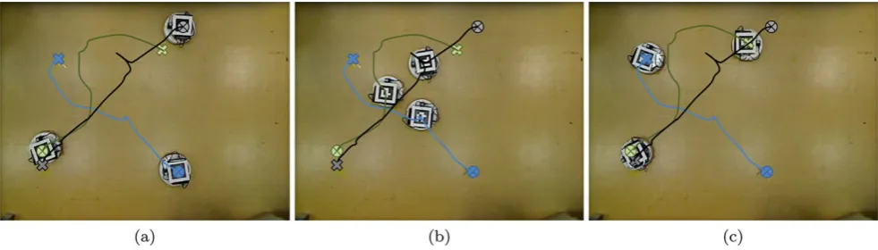
Fig. 7 Real experiment with two robots, with the real path, the initial position (circle), the goal (cross), and obstacles. (a) Image in the initial situation; (b) conflict situation where the paths of both robots intersect; (c) final position

Fig. 8 Map of Robot 1 (blackin Fig.7) in: (a) initial situation; (b) conflict situation, where the paths of both robots intersect; (c) final position

and the goal, as well as the obstacles. Figure7a illustrates the initial configuration in the experiment, and Fig.7c shows the final configuration of the experiment. Figure7b shows a conflict situation, where the path determined by the algo-rithm generated the possibility of collision. Due to the Space Colonization algorithm, both robots recalculate the paths in order to deviate and achieve the goal. The map acquired by each robot is showed in Figs.8and9, respectively. Each of these maps represents approximately the same time instant showed in Fig.7, i.e., the initial position, conflict situation, and final position. The shaded area in yellow represents the allocation of space made by the Space Colonization Algo-rithm at that moment. The Robot 1 is illustrated using black color in Fig.7, i.e., the robot that started in left position and finished in right position. It spent approximately 44 s in its path. Robot 2 is illustrated in blue color and spent approx-imately 56 s in its path. The difference in the elapsed time by each robot is due the distance between the start and goal positions and, mainly, the conflict situation where one robot

has captured markers that allowed it to achieve faster the goal.

The second experiment was performed using three robots without obstacle. In this case, only the robots represent ob-stacles. Figure 10 shows the real environment with three robots, the real path, the initial position, and the goal.

Fig-ure10c shows the final configuration of the experiment.

Fig-ure 10b shows a conflict situation, where the path

Fig. 9 Map of Robot 2 (bluein Fig.7) in: (a) initial situation; (b) conflict situation, where the paths of both robots intersect; (c) final position

Fig. 10 Real experiment with three robots, with the real path, the initial position (circle), and the goal (cross). (a) Image in the initial situation; (b) conflict situation where the paths of all robots intersect; (c) final position

The information exchange was not tested in real robots due to the limited size of the tested area. This exchange gives more information to the robots, making easier to solve the path-planning in this case. Thus, in all real tests, we have disabled the information exchange function.

Notice that the same restrictions that exist in D* are still present at Space D*. A major constraint is the level of gran-ularity associated with space discretization. The Space D* is based on a graph-search algorithm, which is costly for large environments.

Another important restriction of the method is that, in its current implementation, it considers the robots as infinitesi-mal, that is, their bodies are considered points. For proper functioning of the algorithm, it must be ensured that all robots never leave their regions of allocated markers and, as these regions reduce, their movements also decrease. For real robots, the algorithm ensures that the centroid of the robot will never leave the bounded region; however, this can cause problems when the allocated area of a robot is very small.

6 Conclusion

The algorithm Space D* focuses on generating paths over spacious environments, keeping the robot far from dynamic and unknown obstacles (wall, obstacles, and other robots). Thus, the method is applicable in realistic situations where using only the D* does not seem a viable alternative. When compared with other methods of path-planning, like Poten-tial Fields, this algorithm has the advantage of not suffering of local minimums, characteristics inherited from D*.

are greater. It is possible to verify that the greater number of robots in complex environments with exchange of informa-tion allow smaller distances. Furthermore, the reducinforma-tion of the mean velocity of the robots in this context is insignificant compared to the gain obtained in the mean distance travelled by the robots.

The complexity of the algorithm proposed is governed by the execution of D*, that is,O(klog(k)), wherekis the number of markers in the environment. The complexity of the algorithm of exchange of information increases linearly with the number of robotsn, leading anO(n) complexity. Besides that, only a few robots are communicating at each time, because two robots only exchange information when they get close of each other. Therefore, the orders of com-plexity presented and the restriction of the robots commu-nicating with each other at only short distances allow the scalability of the system.

Since the proposed method is decentralized, it is possible that the algorithm fails in specific situations. For example, if two robots meet in a narrow hallway that requires one or the other to reverse its direction. Using the Space Col-onization and D* algorithms, it would be possible that one of the robots determines a reverse direction for a significant distance in order to resolve the conflict. Our method would present the solution described if the diameter of the robots were exactly the width of the corridor, which would be a situation not likely to happen. If there is a small space be-tween the wall of the corridor and the robot, the proposed method will indicate this availability for the other one. Con-sequently, the robots probably would be stagnant because there was not enough space to move. Therefore, we suggest, as a future work, to solve problems related to the bottleneck effect.

For another future work, there is an idea of associating confidence levels with markers and extending the algorithm to work with dynamic obstacles. Another future direction is including in the calculation of markers’ costs and concentra-tion of robots in areas of environment, using exchange of in-formation. It makes possible to find places with higher con-centrations of robots and consequently avoid them. More-over, we intend to make more results in a large environment with more robots in order to consolidate our approach. Acknowledgements This work has been supported by grants from CNPq, FAPERGS, CAPES, and FINEP. The authors would like to thank VerLAB members from DCC-UFMG for their collaboration in real experiments, especially to Mario Campos, Elizabeth da Costa, Gabriel Oliveira, Thiago Sonego, and Rafael Colares.

References

1. Bicho AL, Rodrigues RA, Musse SR, Jung CR, Paravisi M, Maga-lhães LP (2012) Simulating crowds based on a space colonization algorithm. Comput Graph 36(2):70–79

2. Bonert M, Shu LH, Benhabib B (2000) Motion planning for multi-robot assembly systems. Int J Comput Integr Manuf 12:301–310 3. Burgard W, Moors M, Fox D, Simmons R, Thrun S (2000)

Collab-orative multi-robot exploration. In: Proceedings of the IEEE inter-national conference on robotics and automation (ICRA), pp 476– 481

4. Burgard W, Moors M, Stachniss C, Schneider FE (2005) Coordi-nated multi-robot exploration. IEEE Trans Robot 21:376–386 5. Chen J, Li LR (2005) Path planning protocol for collaborative

multi-robot systems. In: Proceedings of the IEEE international symposium on computational intelligence in robotics and automa-tion, pp 721–726

6. Choset H, Burdick JW (1994) Sensor-based planning and nons-mooth analysis. In: Proceedings of the international conference on robotics and automation (ICRA), pp 3034–3041

7. Clark CM, Rock SM, Latombe JC (2003) Dynamic networks for motion planning in multi-robot space systems. In: Proceedings of the international symposium on artificial intelligence, robotics and automation in space (i-SAIRAS)

8. Ferguson D, Stentz A, Field D (2005) An interpolation-based path planner and replanner. In: Proceedings of the international sympo-sium on robotics research (ISRR), pp 1926–1931

9. Fraichard T (1998) Trajectory planning amidst moving obstacles: path-velocity decomposition revisited. J Braz Comput Soc 4(3) 10. Franchi A, Freda L, Oriolo G, Vendittelli M (2009) The

sensor-based random graph method for cooperative robot exploration. IEEE/ASME Trans Mechatron 14:163–175

11. Gerkey BP, Vaughan RT, Howard A (2003) The Player/Stage project: tools for multi-robot and distributed sensor systems. In: Proceedings of the 11th international conference on advanced robotics, pp 317–323

12. Guo Y, Parker LE (2002) A distributed and optimal motion plan-ning approach for multiple mobile robots. In: Proceedings of IEEE international conference on robotics and automation (ICRA), pp 2612–2619

13. Jung JH, Park S, Kim SL (2010) Multi-robot path finding with wireless multihop communications. IEEE Commun Mag 48:126– 132

14. Koenig S, Likhachev M (2002) Improved fast replanning for robot navigation in unknown terrain. In: Proceedings of the international conference on robotics and automation (ICRA), pp 968–975 15. Latombe JC (1991) Robot motion planning. Kluwer Academic,

Dordrecht

16. LaValle SM (2006) Planning algorithms. Cambridge University Press, Cambridge

17. Leroy S, Laumond JP, Simeon T (1999) Multiple path coordina-tion for mobile robots: a geometric algorithm. In: Proceedings of the international joint conference on artificial intelligence (IJCAI), pp 1118–1123

18. Likhachev M, Ferguson DI, Gordon GJ, Stentz A, Thrun S (2005) Anytime dynamic A*: an anytime, replanning algorithm. In: Pro-ceedings of the fifteenth international conference on automated planning and scheduling (ICAPS), pp 262–271

19. Maffei RQ, Botelho SSC, Silveira L, Drews P Jr, Duarte Filho NL, Bicho AL, Almeida FR, Longaray MM (2011) Space D*: um algoritmo para path-planning multi-robôs. In: Proceedings of the VIII ENIA/CSBC, pp 607–618

20. López de Màntaras R, Amat J, Esteva F, López M, Sierra C (1997) Generation of unknown environment maps by cooperative low-cost robots. In: Proceedings of the first international conference on autonomous agents, pp 164–169

22. Pallottino L, Scordio VG, Frazzoli E, Bicchi A (2007) Decentral-ized cooperative policy for conflict resolution in multi-vehicle sys-tems. IEEE Trans Robot 23:1170–1183

23. Parsons D, Canny J (1990) A motion planner for multiple mo-bile robots. In: Proceedings of IEEE international conference on robotics and automation (ICRA), pp 8–13

24. Pereira GAS, Das AK, Kumar V, Campos MFM (2003) Decen-tralized motion planning for multiple robots subject to sensing and communication constraints. In: Proceedings of the second multi-robot systems workshop, pp 267–278

25. Rekleitis IM, Dudek G, Milios EE (1997) Multi-robot exploration of an unknown environment, efficiently reducing the odometry er-ror. In: Proceedings of the fifteenth international joint conference on artificial intelligence, pp 1340–1345

26. Runions A, Fuhrer M, Lane B, Rolland-Lagan PFAG, Prusinkiewicz P (2005) Modeling and visualization of leaf venation patterns. ACM Trans Graph 24:702–711

27. Stentz A (1995) The focussed D* algorithm for real-time replan-ning. In: Proceedings of the international joint conference on arti-ficial intelligence

28. Van den Berg J, Snoeyink J, Lin M, Manocha D (2009) Central-ized path-planning for multiple robots: optimal decoupling into sequential plans. In: Proceedings of the robotics: science and sys-tems (RSS)

29. Van den Berg JP, Ferguson D, Kuffner J (2006) Anytime path-planning and repath-planning in dynamic environments. In: Proceed-ings of the IEEE international conference on robotics and automa-tion (ICRA), pp 2366–2371

30. Wagner D, Schmalstieg D (2007) ARToolKitPlus for pose tracking on mobile devices. In: Proceedings of the 12th computer vision winter workshop (CVWW), pp 139–146

31. Wurm KM, Stachniss C, Burgard W (2008) Coordinated multi-robot exploration using a segmentation of the environment. In: Proceedings of the IEEE/RSJ international conference on intel-ligent robots and systems, pp 1160–1165