Application of variable selection and dimension reduction on predictors of MSE’s development

(1)

Application of variable selection

and dimension reduction on predictors of MSE’s

development

Habtamu Tilaye Wubetie

*

Abstract

Nature create variables using its character component, and variables are sharing characters from a vary small to relatively large scale. This results, variables to have from a vary different to a more similar character, and leads to have a relation ship. Litera-ture suggested different relation measures based on the naLitera-ture of variable and type of relation ship exist. Today, due to having high variety of frequently produced large data size, currently suggested variable filtering and selection methods have gaps to full fill the need. This research desires to fill this gap by comparing literature suggested methods to finding out a better variable selection and dimension reduction methods. The result from regression analysis using all literature suggested factors shows that none of the predictors for development status of enterprise are significant, and only 10 predictors for number of employer in an enterprise are significant out of 81 fac-tors. Since, variable selection and dimension reduction methods are applied to find out predictors of a response by removing variable redundancy, and complexity of incorporating large number variable. Based on statistical power, for the results from variable selection methods, specially association and correlation methods showed that, CANOVA more efficiently detects non-linear or non-monotonic correlation between a continuous–continuous and a continuous-categorical variables. Spearman’s correlation coefficient more efficiently detects a monotonic correlation between a continuous with a continuous, and a continuous with a categorical variable. Pearson correlation coefficient more efficiently detects the linear correlation between continuous vari-ables. MIC efficiently detects non-linear or non-monotonic relation between continu-ous variables. Chi-square test of independence efficiently detects relation between a continuous with a continuous, and categorical with categorical variables, but the non linear or non monotonic relation between a continuous with a categorical are not well detected. On the other hand, the result from lasso and stepwise methods reveals that, the relation between the predictor and response due to interaction effect not detected by correlation and association methods are detected by stepwise variable selection method, and the multicollinearity is detected and removed by lasso method. Regressing the response variable “number of employer in an enterprise” based on vari-ables selected by lasso and stepwise method does bring greater model fitness (based on adjusted R-squared value) than variables selected by association and correlation methods. Similarly, regressing the response variable “development status of an enter-prise” based on variables selected by association and correlation methods does bring

Open Access

(http://creat iveco mmons .org/licen ses/by/4.0/), which permits unrestricted use, distribution, and reproduction in any medium,

provided you give appropriate credit to the original author(s) and the source, provide a link to the Creative Commons license, and indicate if changes were made.

METHODOLOGY

(2)

12 significant variables, where none of variables are significant from variables selected by lasso and stepwise methods. As a result, 51 predictors for number of employment in an enterprise, and 40 predictors for development status of an enterprise are detected as significantly related variables. And, lasso and stepwise methods are preferred to select predictors of a continuous response variable “number of employers in an enter-prise”, and association and correlation methods are preferred to select predictors of a categorical response variable “development status of an enterprise”. Finally, the reduced regression models result reveals that, 20 predictors have causal relation with number of employment in an enterprise, and 12 predictors have causal relation with development status of an enterprise. On the other hand, based on model fitness, information lost, and number of significant factors, principal factor is preferred and applied in dimen-sion reduction for a categorical response variable “development status of an enterprise”, and factor score based regression is preferred and applied for a continuous response variable “number of employers in an enterprise”. However, the comparison of the results in variable selection and dimension reduction indicates that, variable selection methods gave more gain in model fitness than dimension reduction methods. Hence, the suggested variable selection methods are more preferred than dimension reduc-tion methods, and applied to find out predictors. In general, the suggested procedure for variable selection methods are recommended when small number of variables are studied, and the suggested dimension reduction methods are recommended for large number of variant variables (Big data case).

Keywords: Variable selection, Dimension reduction, CANOVA, Stepwise elimination, Lasso variable selection

Introduction

Nature create variables using its character component, and variables are sharing charac-ters from a vary small to relatively large scale. This results, variables to have from a vary different to a more similar character. Variables having a more similar character are vari-ables sharing largely a more similar character component (have relatively the same com-position), and apparently a vary small similarity is due to high difference in component character composition. Hence, taking variables having more similar character as one variable or taking one of them as a representative can remove natural character redun-dancy, and it helps to mange and analyse the relation ship between variables in a world of large amount of variables are inter-related. This inter-relation between the variables causes the variables to have a direct causal relation, or an indirect causal relation or rela-tion with out causal nature. Statistically, a direct causal relarela-tion indicates the presence of dependency between variables, where as indirect causality is due to the presence of latent variable. However, the relation between the variables without known causality is due to not well understood relation in the real world. The relation between variables can be linear or non-linear or random. Statistical methods like, variable-selection and varia-ble-dimension-reduction methods can used to reduce the number of variable by taking single variable or merging as a component for statistically significantly similar variables.

Measuring the predictor–predictor relation, and response–predictor relation is important to recognize the relationship exist, and having a short list of influential factors for further analysis to determine their effect on response variable.

(3)

association or correlation measures only. Correspondingly, this interaction effect is planed to detected for real data using Micro and small enterprise (MSE’s) data set[File Name: MSEs.csv] by considering the predictors filtered by association, correlation and regression measures for predictor–predictor and predictor–response relation. Then, the possible com-bination of selected (filtered) groups of variables are then regressed for response variable, and significantly and potentially related variables are re-selected using stepwise and lasso variable selection method.

Statistical measures of association, correlations and regression are used to find out the relation exist between variables. In this research the statistical relation measures used for variable selection, and dimension reduction are, Pearson correlation coefficient, Spearman’s rank correlation coefficient, Chi-square test of independence, maximal information crite-rion (MIC), continuous analysis of variance test (CANOVA), stepwise variable selection and lasso variable selection, and Principal factor and Factor score analysis respectively.

Wang et al. [20] used simulated and real datasets (kidney cancer RNA-seqdataset) to

compare the false positive rates and statistical power of CANOVA to six other methods (Distance correlation’s, Hoeffding’s independence test, CANOVA the Pearson correlation coefficient, the Spearman’s rank correlation coefficient, the Kendall’s rank correlation coef-ficient and the Maximal information coefcoef-ficient), and showed that CANOVA, the Pearson correlation coefficient, the Spearman’s rank correlation coefficient, the Kendall’s rank cor-relation coefficient and the MIC gave the expected false positives. Hence, these methods can detect the true significant variables. However, the false positive rate is lower than the expected for distance correlation and higher than the expected for Hoeffding’s independ-ence test. So the true significant variables may not be detected by distance correlation, and there may be false significant variables in Hoeffding’s independence test result. Hence, Pearson correlation were recommended when correlation between two continuous variable is linear, and CANOVA were recommended when the correlation between two continuous variable is non-linear or complicated.

Variable dimension reduction is a tool to avoid complexity due to having large number of variables by considering the possible small number of variables those can reflect the needed information: which arise due to some variables are highly correlated to each other or to latent variable, or from the set of variables some variables may accounted for large amount of variability in the data set. For this type of problem variable reduction methods like

prin-cipal factor analysis and factor score analysis are suggested [1, 2].

Currently due to having high variety of frequently produced big data size, literature sug-gested variable filtering and selection methods have gaps to full fill the need. Hence, this research desires to fill this gap by finding out a better variable filtering, selection and dimen-sion reduction methods using real data. The above statistical methods of variable-selection and variable-dimension-reduction are applied to reduce the number of variable by taking single variable or merging as a component for statistically significantly similar variables.

Data and variable

From literature, entrepreneur’s development is measured in relation to the success of

an individual, society, and firm survival [3, 4]. Bosma et al. [4] measured development

(4)

entrepreneurs are dependent on the starting human capital, social capital, financial capi-tal and strategies applied on business.

Coduras et al. [5] construct a measure for an individual’s readiness for

entrepreneur-ship based on three main categories: sociological, psychological and managerial–entre-preneurial. The South African small enterprise development agency perform a study based on literature and current data for the impact of 2008 and 2009 global financial crisis on South Africa’s SMMEs, and they suggests that the South Africa’s SMMEs are challenged by access to finance and markets, poor infrastructure, labour laws, crime,

skills shortages and inefficient bureaucracy. Assefa et al. [7] perform a study on factors

affecting the success of Micro and Small-scale Enterprises in Addis Ababa and five other major regional towns in Ethiopia and find out the key success factors are personal quali-ties, such as having an articulate vision or ambition and innate abiliquali-ties, working experi-ence in the formal sector as a factory employee or having worked in family businesses, managerial and entrepreneurial skills, and higher equity in the invested money. Whereas shortage and small size of credit, shortage of working and sales spaces, lack of rental machinery and stringent licensing requirements are constraints of MSEs.

The sample data is taken from Debre Markos town enterprises in 2017. The study units are individuals starting their business in the interval of a year 1994 to 2006 and currently working on their own enterprise or business. The respondents gave detailed information on their entrepreneurial knowledge, skill and experience, on business environment and their strategies. Additional information on enterprises were also taken from Trade and industry office of Debre Markos town.

Sampling method of a study is determined based on the nature of the population under study. Ethiopian Ministry of Urban Development and Housing (MoUDH) classify micro and small size enterprise into five sectors, namely Manufacturing sector, Service sector, Trade, Construction sector, service sector, and Mining and Quarrying Sector. However, based on the present Trade and industry office of Debre Markos town MSEs are re-clas-sified as Manufacturing sector, Service sector, Trade, Urban farming and Construction sector, by splitting Service sector in to service and Urban Farming. Hence, enterprises across sector are more heterogeneous than within sector, stratified sampling method is the right choice. The sample size is determined by using stratified optimal allocation based on the strata’s variance calculated from the information (secondary data) obtained from Trade and industry office: for the situation in which the variable of interest is enter-prise development status which is categorical with value 1 (achieved expected progress

stated by MoUDH) and 0 (not achieved expected progress), and at 99% level of

confi-dence for the true population proportion to be in 0.05 interval of the sample proportion, 179 sample of enterprise is taken from a total of 2093 enterprises. The study unites are allocated to each strata by considering strata’s variance rather than proportion, due to high difference in strata’s size where some clusters have size less than 20 and some larger

than a thousand [8].

Variable of the study

Under these study two dependent and 81 independent variables are considered. List of

(5)

Dependent variable

The variable of interest is enterprise development status. Bosma et al. [4] measured

Entrepreneurs development (which is individual approach to measure enterprise devel-opment status ) in relation to, the success of an individual like profit made and capital growth, the success of society based on employee capacity, and firm survival. Contextu-ally, Ethiopian Ministry of Urban Development and Housing (MoUDH) state a measure for development status of micro and small size enterprise based on the progress made by an enterprise on their capital accumulation and human capital mainly in terms of

number of employee [3]. The MoUDH definition for micro and small enterprise is given

by Table 1.

Correspondingly, on this study enterprise development status is measured based on the progress made by an enterprise which is a categorical variable with value 1 (achieved expected progress) and 0 (not achieved expected progress), and by number of employers in an enterprise as defined by MoUDH.

Explanatory variables

Explanatory variables or factors those have direct or indirect influences on interest vari-able is the concern need to dig out to find out relevant solution on achieving the planed enterprise development by controlling influential variables. As stated on literature by

Bosma et al. [4] determinants for development of entrepreneurs are related to starting

human capital, social capital, financial capital, and strategies applied on business. In general, literature suggested measures of control variables, human capital, finan-cial capital, influencing factors, sofinan-cial capital, and information’s relevant for the

develop-ment of their businesses are considered [3–19].

Variable‑selection method Chi‑squared test of independence

Chi-square test of independence is one of the statistical measures that tests the linear and non-linear association between variables. This test helps to determine whether variables are independent of each other or whether there is pattern of dependency between variables. Formally, chi square test of independence determine whether the observed pattern between the variables is strong enough to show that the two variables are dependent on each other, or by considering all possible combinations of variables events and testing for the independence of each pair of these events. If the probability of occurrence of the different possible values of one variable depend on which category of another variable occurs, then the two variables are dependent on each other. Chi-square variable have a continuous distribution obtained by the sum of the squares of a set of

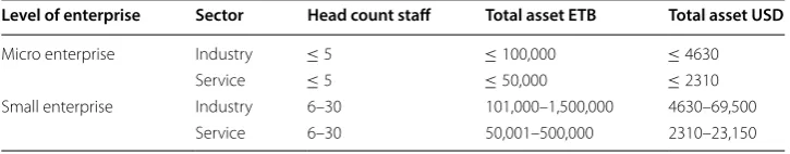
Table 1 Current definition of MSEs in Ethiopia

Level of enterprise Sector Head count staff Total asset ETB Total asset USD

Micro enterprise Industry ≤5 ≤100,000 ≤4630

Service ≤5 ≤50,000 ≤2310

(6)

normally distributed variables. Chi-square distribution is a rightly skewed distribution

with lower limit at 0 and declines as χ2 increases to the right with most of values near

the center of the distribution. Since, theoretical distribution of chi square distribution is a continuous distribution, and the chi square statistic have discrete distribution, chi square statistic is approximated by the theoretical chi square distribution for reasonably large sample size or for expected number of cases exceed 5 in most cells of the cross classification table. The wildly used rule on expected cases are less than 1 and no more than 20% of expected cases have less than 5 per category. The chi square test for inde-pendence is conducted by assuming that there is no relationship (independent) between the two variables being examined versus an alternative hypothesis clam: there is some relationship (dependency) between the variables. Under the null hypothesis of no rela-tionship between variables, the expected cases for each of the cell can be obtained from the multiplication rule of probability for independent events.

Continuous analysis of variance test (CANOVA)

CANOVA is a measure for non linear correlation between two continuous variables, as an extension to ANOVA for continuous variables by making generalization on “within category variance”. CANOVA first define a neighborhood for each data point of response variable based on its predictor value, and then the variance of the response value within the neighborhood is calculated. The hypothesis of CANOVA “similar neighbor predic-tor values lead to similar response values” is tested for smaller value of statistic “within neighborhood sum square” compared to “random expectation”. Since, a statistic “within neighborhood variance” does not follow any familiar distribution, its significance is tested by permutation test. The grid of a larger K has more power on slow-varying func-tions, while a smaller K has more power on quick-oscillating functions depending on

the data. The suggested choice for the neighborhood structure of the dataset is n/20

[20]. CANOVA is related to local regression (like, K nearest neighbor (kNN) regression),

and CANOVA can be viewed as an analogy of the model fitness test of the kNN model as Pearson’s correlation coefficient can be viewed as the model fitness test of a linear regression model. This method reduce algorithm complexity to O(nlogn+np) by order-ing the data values of response with respect to the ordered value of predictors, and can easily explore the non linear correlation between two continuous variable.

Maximal information criterion (MIC)

MIC is an equitable maximal information-based non-parametric exploration (MINE) statistic for identifying and classifying relationships. This implies, in addition to measur-ing association, MIC measures non-linear relation between two random variables, and the degree of linear relation between variables having functional relationships. In gen-eral, with sufficient sample size it captures all type of functional relationships even that are not well modelled. MIC assigns a score measures strength of relationship in a rage of 0 to 1, where a score of 0 to statistically independent variables, and a score of 1 in prob-ability for noiseless functional relationships. For large data set with many variables (Big data) which contain important and undiscovered relationships, MINE helps in identify-ing and characterizidentify-ing structures in data for variable selection or dimension reduction

(7)

Pearson correlation coefficient

The Pearson correlation coefficient is the most commonly used correlation method to measure a two-way linear correlation, calculated by dividing covariance of two variables

by the product of their standard deviations’. Its value is represented by (rxy) in a range

between − 1 and 1. If the points (xi,yi) are in a perfect straight line and the slope of that

line is positive, (rxy)=1 . If the points are in a perfect straight line and the slope is negative,

(rxy)= −1 . If there is no systematic relation between X and Y at all, (rxy)≃ 0, and (rxy)

dif-fers from zero only because of random variation in the sample points.

Coefficient of determination which is the square of Pearson correlation between a

response and an explanatory variable (R2_xy=r_xy2) represents the fraction of the total

var-iance around the mean value y¯ that is explained by the linear relation between xi and y.

Therefore, using (R2

xy) as a variable ranking criterion enforces a ranking according to

good-ness of linear fit of individual variables. However, Pearson correlation measures only linear

dependency between variables [22].

Spearman’s rank correlation coefficient

Spearman’s rank correlation coefficient is non-linear rank based non-parametric test of correlation. Its value is between − 1 and 1 and interpreted in the same way as Pearson cor-relation coefficient for ranked variables. Spearman’s rank corcor-relation coefficient state an alternative hypothesis of the correlation between two variables corresponds to a monotonic function.

Stepwise variable selection

Backward elimination or Forward selection or Stepwise elimination can be used to select variable in the model. Backward elimination starts using all variable and variables with high P-value or above critical value are removed until the rest are significant. Forward selection starts with no variable and the variable not in the model with P-value less than critical value are inserted until the left are not significant. Stepwise elimination is the combination of them, variables are added or removed earlier in the process and the process chose the best collection of variable which maximize model fitness. Stepwise elimination is not exactly dependent on P-value rather it consider the importance of the variable in the model, this results the method to be more power full in prediction. Hence, Stepwise elimination is used to measure the interaction effect of predictors on response variable base on minimum AIC

criterion [23].

Lasso variable selection

Lasso minimises the residual sum of square subject to the sum of the absolute value of the coefficients less than a constant. Lasso is help full to improve prediction accuracy by reduc-ing large variance made by OLS trough shrinkreduc-ing some coefficients to zero. In this study, lasso variable selection method is applied at optimum lambda (which is in range of 1

(8)

Dimension reduction methods Principal factor and factor score analysis

Principal component analysis is helpful to describes the variance-covariance structure between the set of variables through a few uncorrelated new latent variables called princi-pal components. However, the lack of correlation between principrinci-pal components dose not reflect the natural correlation present on represented real variables. Therefore, a method that allow relatively slight correlation between components, like factor analysis, is preferable. fac-tor analysis is can be applied after the number of components needed is decided to construct principal factors and factor scores. The decision for number of principal component needed can be done by considering the bend of the scree plot for principal components variances, the variance or eigenvalue of the principal component greater than one, the proportion of the total variation a counted by principal components, and subject matter consideration

on principal factors composition [1]. The factor model for the random variables vector Y′

= [Y1,Y2,. . .Yp] with mean vector µ and covariance matrix is given as follow:

where is p×k matrix of unknown constants called loadings, F is a k×1 vector of

common factors and ε is a p×p diagonal matrix of specific factors. The estimates

needed from this model are: covariance between factors and variables: Cov(F,Y₎=L

or Cov(Yi,Fj)=l_ij , Communality: h2_i =_jk₌₁l_ij2 , and Uniqueness: φi=Var(Yi)−h2_i for

i, j=1, 2, 3, ...,p.

The ith communality ( h2_i ) indicates the portion of the variance of Yi explained by k

common factors and ith uniqueness ( φ_i ) indicates the portion of variance of Y (Var(Yi) )

explained by the ith specific factors. Estimated principal factors are constructed by linear

combination of variables and their corresponding loadings.

From the result of factor model the estimated factor scores are also constructed by linear combination of original variables having relatively large loading on the factor.

where lij=1 if the variable i have relatively large loading on the factor j, else lij=0 [2].

Model

Linear regression

For the data consist of a random response variable Y (number of employer in an enterprise)

and k = 81 fixed explanatory variables, X1,X2,. . .,Xk with sample of size n = 179, linear

regression is used to fit the parameter estimates and find out influential factors which

deter-mine number of employer in an enterprise. The relationship between Y and X1, X2,. . .,Xk

is formulated as a linear model:

Y=µ+�F+ε,

ˆ

pf_j= p

i=1 lijYi

ˆ fj=

p

i=1

lijYi

(9)

where β0,β1,. . .,βk are constants referred to as regression model coefficients and ǫ is a random disturbance.

It is assumed that Y is approximately a linear function of the X′_s , and _ǫ measures the

discrepancy in that approximation or ǫ contains no systematic information for

determin-ing Y that is not already captured by the X′_s_[₂₅_].

Logistic regression

Enterprise development status is a binary response variable with measured values Y = 1 (achieved expected progress) or Y = 0 (not achieved expected progress). Which is mod-elled by logistic regression model. This model is used to show the relationship between

p(y) and x’s for the random component have binomial distribution where 0≤p(y)≤1.

The mean and variance of the p(y) is np and np(1−p) respectively, where

Logistic regression makes no assumption about the distributions of the independent variables. They do not have to be normally distributed, linearly related or of equal vari-ance with each group. In this study, logistic regression is used to find out the influen-tial factors from suggested predictors of enterprise development status. The influence of determinant factors are assessed individually and component wise on enterprise devel-opment status. It is modelled as follow:

where X is a matrix of independent variable, or principal factors, or factor scores in the

model, β is vector of coefficients of the model, and β0 is intercept of the model [26].

Result and discussion

Linear regression result for the number of employment using all 81 literature suggested

factors showed in Appendix: Tables 12, 13, 14, 15, 16 and 17reveals that only 10

vari-ables are significant (those are, h4, h3, IF4, IF8, Grouping, X15.29, X50.65, ed0, ed1,

and emp_male ) with 0.9992 adjusted R-squared, and similarly the result in Appendix:

Tables 12, 13, 14, 15, 16 and 17 for logistic regression of development status of enterprise

indicates none of the predictors are significant out of 81 factors. To address this problem variable selection and dimension reduction methods are applied to find out the real pre-dictors of a response by removing variable redundancy, and complexity of having large number of variable.

Variable selection

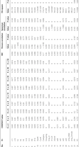
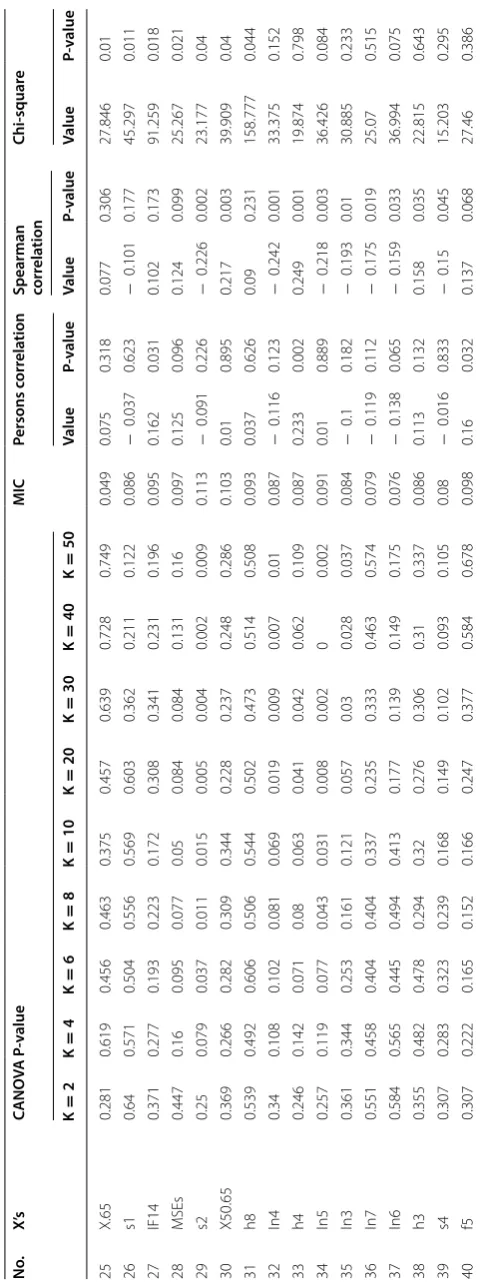
The result of tests for the relation between number of employment in enterprise and

predictors indicated in Table 2 reveals that, number of employers in an enterprise is

sig-nificantly related at 95% confidence level with 40 explanatory variables out of 81

predic-tors listed in Appendix: Tables 12, 13, 14, 15, 16 and 17. Specifically, this result suggested

that, as the number of employer in an enterprise increase, employment by gender is proportional, employment by eduction category is also significantly increased mainly employer with primary education is employed largely, and employment by age category

p(y)= e

β0+β1X1+···+βkXk

1+eβ0+β1X1+···+βkXk

(10)

Table 2 Rela tion b et w een numb er of emplo ymen t in en terprise and e xplana tor y v ariables N o. X’s CANO VA P ‑v alue MIC Persons c orr ela tion

Spearman corr

(11)

Table

2

(c

on

tinued)

N

o.

X’s

CANO

VA P

‑v

alue

MIC

Persons c

orr

ela

tion

Spearman corr

ela

tion

Chi

‑squar

e

K

=

2

K

=

4

K

=

6

K

=

8

K

=

1

0

K

=

2

0

K

=

3

0

K

=

4

0

K

=

5

0

Value

P‑

value

Value

P‑

value

Value

P‑

value

25

X.65

0.281

0.619

0.456

0.463

0.375

0.457

0.639

0.728

0.749

0.049

0.075

0.318

0.077

0.306

27.846

0.01

26

s1

0.64

0.571

0.504

0.556

0.569

0.603

0.362

0.211

0.122

0.086

−

0.037

0.623

−

0.101

0.177

45.297

0.011

27

IF14

0.371

0.277

0.193

0.223

0.172

0.308

0.341

0.231

0.196

0.095

0.162

0.031

0.102

0.173

91.259

0.018

28

MSEs

0.447

0.16

0.095

0.077

0.05

0.084

0.131

0.16

0.097

0.125

0.096

0.124

0.099

25.267

0.021

29

s2

0.25

0.079

0.037

0.011

0.015

0.005

0.004

0.002

0.009

0.113

−

0.091

0.226

−

0.226

0.002

23.177

0.04

30

X50.65

0.369

0.266

0.282

0.309

0.344

0.228

0.237

0.248

0.286

0.103

0.01

0.895

0.217

0.003

39.909

0.04

31

h8

0.539

0.492

0.606

0.506

0.544

0.502

0.473

0.514

0.508

0.093

0.037

0.626

0.09

0.231

158.777

0.044

32

In4

0.34

0.108

0.102

0.081

0.069

0.019

0.009

0.007

0.01

0.087

−

0.116

0.123

−

0.242

0.001

33.375

0.152

33

h4

0.246

0.142

0.071

0.08

0.063

0.041

0.042

0.062

0.109

0.087

0.233

0.002

0.249

0.001

19.874

0.798

34

In5

0.257

0.119

0.077

0.043

0.031

0.008

0.002

0

0.002

0.091

0.01

0.889

−

0.218

0.003

36.426

0.084

35

In3

0.361

0.344

0.253

0.161

0.121

0.057

0.03

0.028

0.037

0.084

−

0.1

0.182

−

0.193

0.01

30.885

0.233

36

In7

0.551

0.458

0.404

0.337

0.235

0.333

0.463

0.574

0.079

−

0.119

0.112

−

0.175

0.019

25.07

0.515

37

In6

0.584

0.565

0.445

0.494

0.413

0.177

0.139

0.149

0.175

0.076

−

0.138

0.065

−

0.159

0.033

36.994

0.075

38

h3

0.355

0.482

0.478

0.294

0.32

0.276

0.306

0.31

0.337

0.086

0.113

0.132

0.158

0.035

22.815

0.643

39

s4

0.307

0.283

0.323

0.239

0.168

0.149

0.102

0.093

0.105

0.08

−

0.016

0.833

−

0.15

0.045

15.203

0.295

40

f5

0.307

0.222

0.165

0.152

0.166

0.247

0.377

0.584

0.678

0.098

0.16

0.032

0.137

0.068

27.46

(12)

is significantly increased for category between 30–49 and 50–65. But, the number of employer between age category 15 to 29 is decreases as the number of employer in an enterprise increases. Enterprise created by group, employer taking specific education or training on entrepreneurship, employer graduate from TVET are significantly directly correlated with the growth of enterprise’s employability. Apparently, having relation with entrepreneurs for advise like as friend and any one in contact is negatively correlated with number of employment in an enterprise. The result also indicate current capital and Government investment policy motivation by Land are significantly directly correlated with number of employment in an enterprise. The influence of religion, traditionalism (cultural tackle), problems related to the legal licensing, telecommunication problems, and lack of necessary and timely marketing information have significant direct correla-tion with the number of employers in an enterprise. The problem of keep up with litera-ture, get information from customers, get information from suppliers, get information from banks, and get information from commercial cooperation is higher as number of employment in an enterprise increases. The development status of an enterprise have significant have negative correlation with the number of employers in an enterprise. In addition, Starting capital, educational level, experience in self-employment, manage-rial experience, financial experience (financing the business), experience in the sector, firm duration, experience in business, corruption, number of employers on age category above 65, having entrepreneurs in the family, type of MSEs (micro or small), and expe-rience as an employee have significant association with number of employment in an enterprise.

CANOVA helps to detect the relation exist between a continuous and categorical

vari-able (only CANOVA with k = 10 detects type of MSEs has significant correlation with

number of employment in an enterprise increases, and CANOVA have high power to detect the correlation exist between In5 (get information from suppliers) and number of employment in an enterprise increases). However, almost all significant variables detected by CANOVA are detected by Pearson or Spearman’s correlation coefficient, mainly by Spearman’s correlation coefficient. MIC also detects some non linear

rela-tion between some continuous variable with high power (Currk, Emp0 , X15.29, X30.49,

emp_male , and emp_Female.

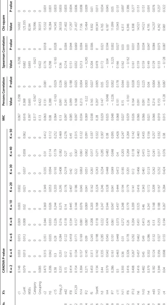
The result of tests for the relation between the development status of an enterprise and

explanatory variables indicated in Table 3 reveals that, the development status of

enter-prise is significantly related at 95% confidence level with 28 explanatory variables out

of 81 predictors listed in Appendix: Tables 12, 13, 14, 15, 16 and 17. This result

(13)

(14)

and even at the start-up. The development of an micro enterprise enterprise is better than small enterprise. There is also an evidence of starting a business in group could bring a better development than an individual owned business, similarly male owned enterprises are more successful. Government investment policy motivation by land has also direct significant correlation with development of an enterprise. So government investment policy motivation is helpful for success of an enterprise. Having experience in the sector (your business), financial experience (financing the business), working by business plan, employment growth goal (the desire/want to employee), managerial skills, and experience in business have direct significant correlation with development of an enterprise. Mainly, formal managerial skills and financial experience have significant correlation with the development of an enterprise. In addition, bad experience of own have significant association with the development of an enterprise. The result indicated

that, only CANOVA for k = 2 find out entrepreneurs activeness on business services

is significantly negatively correlated with development status of an enterprise. MIC detected some non-linear relation with high power (Currk, MSEs, and Category). How-ever, almost all significant variables detected by CANOVA are detected by Pearson or Spearman’s correlation coefficient, mainly by Spearman’s correlation coefficient.

Conclusion based on statistical power, the result from association and correlation

analysis suggested that, CANOVA more efficiently detects continuous–continuous, and continuous-categorical non-linear or non-monotonic relation. Spearman’s correlation coefficient more efficiently detects a continuous–continuous or a continuous-categori-cal monotonic relationship. Pearson correlation coefficient more efficiently detects the relation between continuous variables. MIC more efficiently detects linear or non-monotonic continuous-continuous relation. Chi-square test of independence efficiently detects relation between a continuous with a continuous, and categorical with categori-cal variables, but the non linear or non monotonic relation between a continuous with a categorical are not well detected. On the other hand, the results from stepwise and lasso

variable selection method in Table 5 shows that, 31 variables are detected significantly

as predictor for number of employment in an enterprise, and from which eleven of them are new predictors comparing to the result in association and correlation methods given

in Table 2. The result using this method in Table 7 also indicates that 21 variables are

sig-nificantly detected as predictors for development status of an enterprise and from which eleven of them are new predictors comparing to the result in association and correlation

methods given in Table 3. Since, association and correlation can not detect the relation

due to interaction effect. Similarly, some of non-causal relation between a predictor and response are not detected by lasso and stepwise variable selection methods are detected by correlation and association methods. Specifically, twenty new variables are selected as predictor for number of employment in an enterprise and nineteen new variables are selected as predictor for development status of an enterprise.

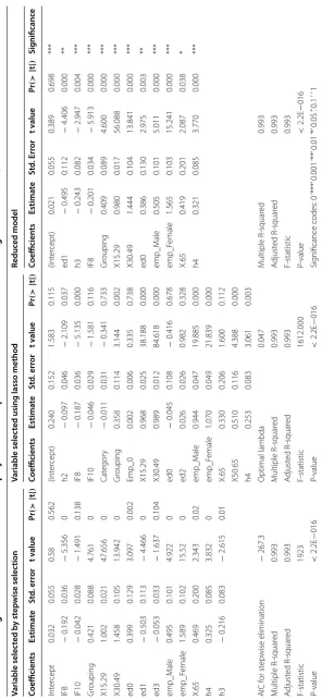
Model result from selected variables Linear regression

1. Influencing factors affecting number of employment in an enterprise are assessed based on casual linear relation with significantly related (correlated or/union

(15)

elimination with minimum AIC criterion, and by lasso variable selection method. Stepwise elimination bring less number of significant variables comparing to lasso variable selection. However, both method have their own input, stepwise elimina-tion brings three new variables (ed1, ed3, h3) those are not significant by lasso,

and lasso method also brings five new variables (h2, Category, Emp0 , ed2, number

of employer from 50 to 65 ) those are not significant by stepwise elimination. The

selected variables by both methods are separately modelled, and the result in Table 4

reveals IF8, grouping, number of employer from age 15–29 and 30–49, emp_male ,

emp_female , and h4 are significant for both methods, where ed0, ed1, h3, and num-ber of employer aged above 65 are only significant by stepwise elimination, similarly h2 and number of employer from age from 50 to 65 are only significant by lasso method. Finally, the variables selected by both methods are merged and the result for reduced model reveals a greater number of significant variables with equivalent

model fitness as indicated in Table 4. The significance of all variables included in

reduced model, unlike the lasso and stepwise selected variables, is an indication of lower multicollinearity between incorporated variables. This implies that, the pre-dictors of number of employment in an enterprise should be the selected variable in reduced model.

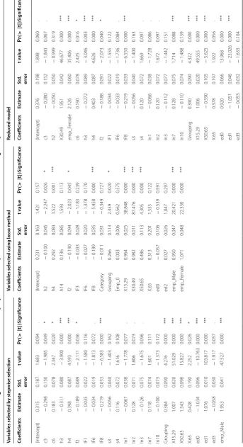
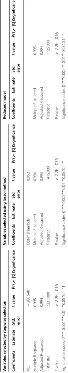
2. Here, influencing factors affecting number of employment in an enterprise

are assessed using all literature suggested factors in Table 5 by regression method

(stepwise elimination and lasso variable selection). Significant factors are selected based on Stepwise elimination with minimum AIC criterion, and by lasso variable selection method at optimum lambda (which is in range of 1 standard deviation of

minimum lambda). Unlike, the above result Table 4, regression of variables selected

by stepwise elimination brings more number of significant variables comparing to variables selected by lasso method. However, both method have their own input in variable selection, stepwise elimination bring threaten new variables (c3, c6, h3, IF1, s3, s4, In1, In2, In3, In7, In10, ed1, and ed3), where five of them are not sig-nificant, but the removal of insignificant variables (IF1, s3, s4, In7 and In10) result in reduction of multiple R-squared and adjusted R-squared from 0.9946 to 0.9942, and 0.9937 to 0.9935 respectively. In addition, two significant variables In1 and In3 become insignificant. So these variables are potential variable and have to stay in the model. On the other hand, lasso method brings eight new variables (h2, h14,

IF3, Category, Emp0 , X30.49, ed2, emp_female ) of which three of them are only

sig-nificant. The removal of insignificant variables (h14, IF3, Category, Emp0 , and ed2),

resulted in reduction of multiple R-squared and adjusted R-squared from 0.9938 to 0.9932, and 0.9931 to 0.9928 respectively. However, there is no significant variable became insignificant due to the removal of those variables. This is an indication that stepwise elimination considers the gain due to interaction effect but it can result in multicollinearity, where as lasso method removes multicollinearity and the gain due to interaction effect is not considered. Due to the advantages of lasso method on controlling multicollinearity and stepwise elimination in considering interaction effect, variables selected by both stepwise elimination and lasso method are merged, and the result for reduced model reveals a greater number of significant variables

(16)

Table 4 Linear r egr ession r esult f or numb er of emplo yer in an en

terprise based on selec

ted fac

tors thr

ough asso

cia

tion or/union c

orr ela tion metho ds Variable selec ted b y st ep wise selec tion Variable selec

ted using lasso method

Reduc ed model Coefficien ts Estima te St d. err or t v alue Pr (> | t | ) Coefficien ts Estima te St d. err or t v alue Pr (> | t | ) Coefficien ts Estima te St d. Err or t v alue Pr (> | t | ) Sig nificanc e Int er cept 0.032 0.055 0.58 0.562 (Int er cept) 0.240 0.152 1.583 0.115 (Int er cept) 0.021 0.055 0.389 0.698 *** IF8 − 0.192 0.036 − 5.356 0 h2 − 0.097 0.046 − 2.109 0.037 ed1 − 0.495 0.112 − 4.406 0.000 ** IF10 − 0.042 0.028 − 1.491 0.138 IF8 − 0.187 0.036 − 5.135 0.000 h3 − 0.243 0.082 − 2.947 0.004 *** Gr ouping 0.421 0.088 4.761 0 IF10 − 0.046 0.029 − 1.581 0.116 IF8 − 0.201 0.034 − 5.913 0.000 *** X15.29 1.002 0.021 47.656 0 Cat egor y − 0.011 0.031 − 0.341 0.733 Gr ouping 0.409 0.089 4.600 0.000 *** X30.49 1.458 0.105 13.942 0 Gr ouping 0.358 0.114 3.144 0.002 X15.29 0.980 0.017 56.088 0.000 *** ed0 0.399 0.129 3.097 0.002 Emp_0 0.002 0.006 0.335 0.738 X30.49 1.444 0.104 13.841 0.000 *** ed1 − 0.503 0.113 − 4.466 0 X15.29 0.968 0.025 38.188 0.000 ed0 0.386 0.130 2.975 0.003 ** ed3 − 0.053 0.033 − 1.637 0.104 X30.49 0.989 0.012 84.618 0.000 emp_M ale 0.505 0.101 5.011 0.000 *** emp_M ale 0.495 0.101 4.922 0 ed0 − 0.045 0.108 − 0.416 0.678 emp_F emale 1.565 0.103 15.241 0.000 *** emp_F emale 1.589 0.102 15.52 0 ed2 0.026 0.026 0.982 0.328 X.65 0.419 0.201 2.087 0.038 * X.65 0.469 0.200 2.343 0.02 emp_M ale 0.944 0.047 19.885 0.000 h4 0.321 0.085 3.770 0.000 *** h4 0.325 0.085 3.832 0 emp_F emale 1.070 0.049 21.839 0.000 h3 − 0.216 0.083 − 2.615 0.01 X.65 0.330 0.206 1.600 0.112 X50.65 0.510 0.116 4.388 0.000 h4 0.253 0.083 3.061 0.003 AIC f or st ep wise elimination − 267.3 Optimal lambda 0.047 M ultiple R-squar ed 0.993 M ultiple R-squar ed 0.993 M ultiple R-squar ed 0.993 A djust ed R-squar ed 0.993 A djust ed R-squar ed 0.993 A djust ed R-squar ed 0.993 F-statistic 0.993 F-statistic 1923 F-statistic 1612.000 P-value < 2.2E − 016 P-value < 2.2E − 016 P-value < 2.2E − 016 Sig

nificance codes: 0

‘***’ 0.001 ‘**’ 0.01 ‘*’ 0.05 ‘.’ 0.1

(17)

Table 5 Linear r egr ession f or the numb er of emplo yer in an en

ted fac

tors thr

ough st

ep

wise elimina

tion and lasso metho

ds Variables selec ted b y st ep wise selec tion Variables selec

(18)

Table

5

(c

on

tinued)

Variables selec

ted b

y st

ep

wise selec

tion

Variables selec

Reduc

ed model

Coefficien

ts

Estima

te

St

d.

err

or

t v

alue

Pr

(>

|

t

|

)

Sig

nificanc

e

Coefficien

ts

Estima

te

St

d.

err

or

t v

alue

Pr

(>

|

t

|

)

Sig

nificanc

e

Coefficien

ts

Estima

te

St

d.

err

or

t v

alue

Pr

(>

|

t

|

)

Sig

nificanc

e

AIC

−

280.540

Optimal lambda

0.052

M

ultiple R-squar

ed

0.995

M

ultiple R-squar

ed

0.994

M

ultiple R-squar

ed

0.995

A

djust

ed R-squar

ed

0.994

A

djust

ed R-squar

ed

0.993

A

djust

ed R-squar

ed

0.994

F-statistic

1231.000

F-statistic

1415.000

F-statistic

1125.000

P-value

<

2.2E

−

016

P-value

<

2.2E

−

016

P-value

<

2.2E

−

016

Sig

nificance codes: 0

‘***’

0.001

‘**’

0.01

‘*’

0.05

‘.’ 0.1

‘ ’ 1

Sig

nificance codes: 0

‘***’

0.001‘**’

0.01

‘*’

0.05

‘.’ 0.1

‘ ’1

Sig

nificance codes: 0

‘***’

0.001

‘**’

0.01

‘*’

0.05

‘.’ 0.1

(19)

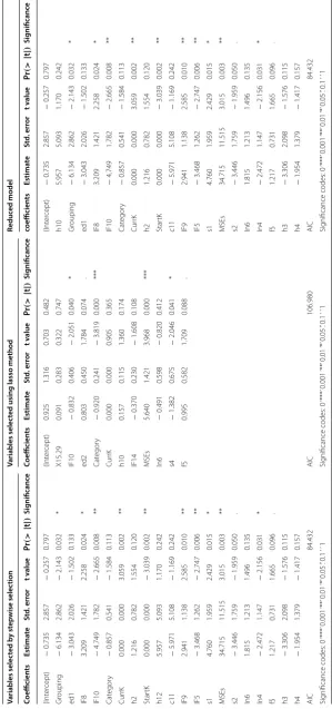
1. Influencing factors affecting development status of an enterprise are assessed based on casual relation of significantly related (correlated or/union associated) predictors

Table 3. Significant variables in the model are selected based on stepwise elimination

with minimum AIC criterion, and lasso method at minimum lambda. Stepwise elimina-tion does brings more variables at lower AIC than lasso method. However, both method have their own input in variable selection, stepwise elimination bring 14 new variables and of eight of them are significant variables (Grouping, IF8, StartK, IF9, IF5, s1, s2, and

In4), and lasso method does bring six new variables (X15.29, ed2, h10, IF14, and s4). The

variables selected by both methods are merged and the result for reduced model reveals a greater number of variables in the model with equivalent model fitness as indicated

in Table 6, and reflects that, Grouping, IF8, IF10, CurrK, StartK, IF9, IF5, s1, MSEs, s2,

In4, and f5 are significant factors on development status of an enterprise where ed1, Cat-egory, h2, h10, c11, In6, h3, and h4 are potential factors.

2. Influencing factors affecting development status of an enterprise are assessed using

all literature suggested factors Table 7. Significant variables in the model are selected

based on stepwise elimination at minimum AIC criterion, and by lasso variable selection method at minimum lambda. As a result stepwise elimination does brings more vari-ables at lower AIC than lasso method. However, predictors selected by lasso method are only significant. The result for reduced model contains more variable with lower AIC, but none of the variables are significant. Hence, lasso variable selection dose in better power.

As conclusion Comparison of the results for reduced linear regressions model of

vari-ables selected by association and correlation method Table 4 with variables selected by

regression method Table 5 revealed that, the earlier method does bring one new variable

( emp_male ) and the latter one does bring eight new variables (those are, IF6, X50.65,

c3, c6, In1, In2, In3, and In7) with greater adjusted R-squared. This reveals that, based on the number of significant variables and model fitness (based on adjusted R-squared value), variables selected by lasso and stepwise elimination are taken as predictors of

number of employer in an enterprise, those are listed on Table 5. Specifically, number

of employer in an enterprise has significant casual relation with full self-employment, previous habitat is urban, Graduated from TVET, taken specific education/training on entrepreneurship, having other income source, environmental conditions, religion, con-tact with entrepreneurs in networks may be socially, visiting Bazaar, taking businesses courses, reading literatures on business, get information about business from commer-cial cooperation, Working MSEs in group, employers with education back ground who can not read and write, and who complete primary education, high females employment, high number of employer age between 15 to 29, 30 to 49, and above 65, and low number of employer aged between 50 to 65.

On the other hand, for categorical response variable “development status of an

enter-prise” the result in Tables 6 and 7 indicates that, more significant number of variables

are find out by association and correlation methods, where non of variables are signif-icant by lasso and stepwise methods with some more AIC value (with more informa-tion lost). Hence, the predictors for development status of an enterprise are variables

(20)

Table 6 L ogistic r egr ession f or de velopmen t sta tus of an en

ted fac

tors thr

ough asso

cia

tion or/union c

orr ela tion metho ds Variables selec ted b y st ep wise selec tion Variables selec

Reduc ed model Coefficien ts Estima te St d. err or t v alue Pr (> | t | ) Sig nificanc e Coefficien ts Estima te St d. err or t v alue Pr (> | t | ) Sig nificanc e coefficien ts Estima te St d. err or t v alue Pr (> | t | ) Sig nificanc e (Int er cept) − 0.735 2.857 − 0.257 0.797 (Int er cept) 0.925 1.316 0.703 0.482 (Int er cept) − 0.735 2.857 − 0.257 0.797 Gr ouping − 6.134 2.862 − 2.143 0.032 * X15.29 0.091 0.283 0.322 0.747 h10 5.957 5.093 1.170 0.242 ed1 − 3.043 2.026 − 1.502 0.133 IF10 − 0.832 0.406 − 2.051 0.040 * Gr ouping − 6.134 2.862 − 2.143 0.032 * IF8 3.209 1.421 2.258 0.024 * ed2 0.803 0.450 1.784 0.074 . ed1 − 3.043 2.026 − 1.502 0.133 IF10 − 4.749 1.782 − 2.665 0.008 ** Cat egor y − 0.920 0.241 − 3.819 0.000 *** IF8 3.209 1.421 2.258 0.024 * Cat egor y − 0.857 0.541 − 1.584 0.113 Cur rK 0.000 0.000 0.905 0.365 IF10 − 4.749 1.782 − 2.665 0.008 ** Cur rK 0.000 0.000 3.059 0.002 ** h10 0.157 0.115 1.360 0.174 Cat egor y − 0.857 0.541 − 1.584 0.113 h2 1.216 0.782 1.554 0.120 IF14 − 0.370 0.230 − 1.608 0.108 Cur rK 0.000 0.000 3.059 0.002 ** Star tK 0.000 0.000 − 3.039 0.002 ** MSEs 5.640 1.421 3.968 0.000 *** h2 1.216 0.782 1.554 0.120 h12 5.957 5.093 1.170 0.242 In6 − 0.491 0.598 − 0.820 0.412 Star tK 0.000 0.000 − 3.039 0.002 ** c11 − 5.971 5.108 − 1.169 0.242 s4 − 1.382 0.675 − 2.046 0.041 * c11 − 5.971 5.108 − 1.169 0.242 IF9 2.941 1.138 2.585 0.010 ** f5 0.995 0.582 1.709 0.088 . IF9 2.941 1.138 2.585 0.010 ** IF5 − 3.468 1.262 − 2.747 0.006 ** IF5 − 3.468 1.262 − 2.747 0.006 ** s1 4.760 1.959 2.429 0.015 * s1 4.760 1.959 2.429 0.015 * MSEs 34.715 11.515 3.015 0.003 ** MSEs 34.715 11.515 3.015 0.003 ** s2 − 3.446 1.759 − 1.959 0.050 . s2 − 3.446 1.759 − 1.959 0.050 . In6 1.815 1.213 1.496 0.135 In6 1.815 1.213 1.496 0.135 In4 − 2.472 1.147 − 2.156 0.031 * In4 − 2.472 1.147 − 2.156 0.031 * f5 1.217 0.731 1.665 0.096 . f5 1.217 0.731 1.665 0.096 . h3 − 3.306 2.098 − 1.576 0.115 h3 − 3.306 2.098 − 1.576 0.115 h4 − 1.954 1.379 − 1.417 0.157 h4 − 1.954 1.379 − 1.417 0.157 AIC 84.432 AIC 106.980 AIC 84.432 Sig

nificance codes: 0

‘***’ 0.001 ‘**’ 0.01 ‘*’ 0.05 ‘.’ 0.1

‘ ’ 1

Sig

nificance codes: 0

‘***’ 0.001 ‘**’ 0.01 ‘*’ 0.05 ‘.’ 0.1

‘ ’ 1

Sig

nificance codes: 0

‘***’ 0.001 ‘**’ 0.01 ‘*’ 0.05 ‘.’ 0.1

(21)

Table 7 L ogistic r egr ession f or de velopmen t sta tus of an en

ted fac

tors thr

ough st

ep

wise elimina

tion and lasso metho

ds Variables selec ted b y st ep wise selec tion Variables selec

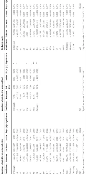
Reduc ed model Coefficien ts Estima te St d. Err or L v alue Pr (> | t | ) Sig nificanc e Coefficien ts Estima te St d. err or t v alue Pr (> | t | ) Sig nificanc e Coefficien ts Estima te St d. err or t v alue Pr (> | t | ) Sig nificanc e (Int er cept) − 322.676 68577.647 − 0.005 0.996 (Int er cept) 1.905 0.956 1.993 0.046 * (Int er cept) − 954.150 32304.935 − 0.030 0.976 c1 − 552.518 33988.886 − 0.016 0.987 c1 − 1.710 0.691 − 2.473 0.013 * IF10 − 461.056 15,574.685 − 0.030 0.976 c5 289.965 20,527.088 0.014 0.989 h5 0.569 0.431 1.319 0.187 c1 − 1,131.226 38,004.669 − 0.030 0.976 h1 11.445 778.170 0.015 0.988 IF7 − 0.121 0.212 − 0.569 0.569 c5 605.125 20,639.885 0.029 0.977 h4 − 455.053 28,358.289 − 0.016 0.987 IF10 − 0.586 0.258 − 2.275 0.023 * h1 18.827 664.254 0.028 0.977 h5 356.473 22,839.877 0.016 0.988 IF13 − 0.572 0.294 − 1.947 0.052 . h4 − 655.461 22,483.411 − 0.029 0.977 h6 − 136.468 8857.694 − 0.015 0.988 MSEs 6.475 1.542 4.199 0.000 *** h5 654.079 22,067.031 0.030 0.976 h7 142.049 9688.991 0.015 0.988 Cat egor y − 0.905 0.21b − 4.217 0.000 *** h6 − 230.180 8704.315 − 0.026 0.979 IF3 147.569 12506.807 0.012 0.991 h7 281.038 10105.656 0.028 0.978 IF9 − 202.959 13861.819 − 0.015 0.988 IF3 237. 720 7991.684 0.030 0.976 IF11 74.875 5115.008 0.015 0.988 IF11 224.844 7969.311 0.028 0.977 IF13 − 365.188 21395.708 − 0.017 0.986 IF13 − 543.842 18109.693 − 0.030 0.976 IF17 112.401 9559.584 0.012 0.991 IF17 151.610 5265.601 0.029 0.977 s1 182.913 22360.952 0.008 0.993 s1 510.642 17258.235 0.030 0.976 s3 − 393.450 36930.442 − 0.011 0.991 s3 − 987.537 33036.343 − 0.030 0.976 Star tK 0.001 0.102 0.014 0.989 MSES 4482.055 152684.795 0.029 0.977 MSEs 1662.705 98798.058 0.017 0.987 Cat egor y − 666.719 22782.652 − 0.029 0.97 7 Cat egor y − 364.239 21327.956 − 0.017 0.986 Gr ouping − 524.788 18505.604 − 0.028 0.977 Gr ouping − 418.374 27113.658 − 0.016 0.988 X15.29 141.460 4728.631 0.030 0.976 X15.29 75.706 4414.207 0.017 0.986 AIC 40.000 AIC 104.460 AIC 38.000 Sig

nificance codes: 0

‘***’ 0.001 ‘**’ 0.01 ‘*’ 0.05 ‘.’ 0.1

‘ ’ 1

Sig

nificance codes: 0

‘***’ 0.001 ‘**’ 0.01 ‘*’ 0.05 ‘.’ 0.1

‘ ’ 1

Sig

nificance codes: 0

‘***’ 0.001 ‘**’ 0.01 ‘*’ 0.05 ‘.’ 0.1

(22)

relation with working MSEs in group, religion, telecommunication problems, tradition-alism (cultural tackle), current capital, corruption, entrepreneurs in the family, entre-preneurs in the friends, get information from customers, government investment policy motivation by land, and status of MSEs is being small. The development of an enterprise status is potentially related with employers with primary education, category of MSEs, year of experience in business, environmental conditions, educational level, Graduated from TVET, Specific education/training on entrepreneurship, and financial experience (financing the business).

Hence, lasso and stepwise variable selection methods are suggested for continuous response variable, and association and correlation methods are suggested for categorical response variable; or alternatively, variable selection method by combing both associa-tion, correlaassocia-tion, and regression method can bring a better result.

Dimension reduction

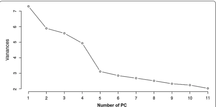
Explanatory factor analysis were applied using varimax rotation on principal compo-nents to reduce variable dimension for a purpose of avoiding complexity due to hav-ing large number of variables with out loshav-ing the needed information. Based on a result

indicated in Appendix: Tables 12, 13, 14, 15, 16 and 17, 11 principal components each

having a minimum of variance equal to 2, which accounts for 50.8% of the total vari-ation in data set were taken by considering the subject matter and the bend point of a

scree-plot of principal components shown in Fig. 1 too. And then, factor elements with

at least 0.3 score (loading) are selected. Specifically, Factor 1 is related to Human and starting capital, Factor 2 contrasts potential input of an enterprise with influencing fac-tors, Factor 3 contrasts an enterprise getting information from partners with an idolised enterprise, Factor 4 is related to knowledge on business mainly by training, education or courses, Factor 5 contrasts own business input with partner support, Factor 6 contrasts policy related influencing functors to Human capital, Factor 7 contrasts Entrepreneurs act for success of an enterprise with Entrepreneurs social resource, Factor 8 related to number of employer in an enterprise per categories of gender, education, and age, Factor

(23)

9 contrasts own contribution with partners, Factor 10 contrasts entrepreneurs nature with enterprise status, Factor 11 contrasts number of employers per category with entre-preneurs potential.

Model result for dimension reduction Linear regression

The linear regression result for the number of employer in an enterprise based on factor

scores reveals Table 8, factor 5 (contrasts of own business input with partner support),

factor 6 (contrasts of policy related influencing functors to Human capital), factor 8 (var-iables related to Number of employer in an enterprise per categories of gender), factor 10 (contrasts of entrepreneurs nature with enterprise status), and factor 11 (contrasts number of employers per category with entrepreneurs potential) have significant affect on number of employer in an enterprise and those factors explain 82% of the variation in mean number of employer in an enterprise.

The linear regression result for number of employer in an enterprise based on

prin-cipal factor reveals Table 9, principal factor 5 (contrasts of own business input with

partner support), principal factor 6 (contrasts of policy related influencing functors to human capital), principal factor 7 (contrasts entrepreneurs act for success of an enter-prise with entrepreneurs social resource), principal factor 9 (contrasts own contribution with partners), principal factor 10 (contrasts of entrepreneurs nature with enterprise sta-tus), and principal factor 11 (contrasts number of employers per category with entre-preneurs potential) are the significant factors those explain 85% of the variation in mean number of employer in an enterprise.

The result from regression analysis using facto score and principal factor indi-cates that regression analysis using principal factor gain more model fitness with one more factor. Even though, four factors are significant by both methods, factor 8 is

Table 8 Linear regression of number of employer in an enterprise based on factor scores

Full model Reduced model by stepwise elimination

Coefficients Estimate Std.

error t value Pr(

>|t|) Coefficients Estimate Std. error t value Pr(>|t|)

(Intercept) 0.762 1.441 0.529 0.597 (Intercept) 1.133 0.706 1.605 0.110

x1 − 0.002 0.013 − 0.115 0.909 x1 Removed

x2 0.007 0.013 0.528 0.598 x2 Removed

x3 0.042 0.082 0.516 0.606 x3 Removed

x4 0.000 0.000 0.442 0.659 x4 Removed

x5 − 0.257 0.026 − 10.063 0.000 x5 − 0.257 0.025 − 10.269 0.000

x6 0.245 0.022 11.289 0.000 x6 0.243 0.021 11.575 0.000

x7 0.014 0.096 0.144 0.886 x7 Removed

x8 0.936 0.067 13.954 0.000 x8 0.938 0.065 14.354 0.000

x9 − 0.106 1.070 − 0.099 0.921 x9 Removed

x10 0.000 0.000 1.864 0.064 x10 0.000 0.000 2.019 0.045

x11 0.066 0.025 2.623 0.010 x11 0.065 0.024 2.667 0.008

Multiple R-squared 0.821 Multiple R-squared 0.820

Adjusted R-squared 0.810 Adjusted R-squared 0.815

F-statistic 69.820 F-statistic 158.000

(24)

only significant by factor score based regression, and factor 7 and 9 are only signifi-cant by principal factor based regression. Since, the result from principal factor based regression brings little gain in model fitness with complex composition (since it con-sider all variables than factor scores, that makes difficult to relate principal factors to real component) comparing to factor score based regression, the factor score based regression is more preferable.

The logistic regression result for development status based on factor score reveals

Table 10, factor 4 (related to knowledge on business mainly by training), factor 7

(contrasts Entrepreneurs act for success of an enterprise with Entrepreneurs social resource), and factor 10 (contrasts of entrepreneurs nature with enterprise status) are the significant factors with AIC of 183.16.

The logistic regression result for principal factor of development status reveals

Table 11, principal factor 2 (contrasts potential input of an enterprise with

Influenc-ing factors), principal factor 3 (contrasts an enterprise gettInfluenc-ing information from part-ners with an idolised enterprise), principal factor 8 (Variables related to Number of employer in an enterprise per categories of gender), principal factor 9 (contrasts own contribution with partners), principal factor 10 (contrasts of entrepreneurs nature with enterprise status), and principal factor 11 (contrasts number of employers per category with entrepreneurs potential) are the significant factors with AIC of 128.348.

The result from logistic regression analysis using factor score and principal fac-tor indicates that logistic regression analysis using principal facfac-tor brings more sig-nificant factors. Principal factor based logistic regression give 6 sigsig-nificant factors, where factor score based logistic regression brings 3 significant factors with lower Table 9 Linear regression of number of employer in an enterprise based on principal factors

Coefficients Estimate Std. error t value Pr(>|t|) Coefficients Estimate Std. error t value Pr(>|t|)

(Intercept) 0.762 1.441 0.529 0.597 (Intercept) 0.793 0.284 2.788 0.006

x1 − 0.002 0.013 − 0.115 0.909 x1 Removed

x2 0.007 0.013 0.528 0.598 x2 Removed

x3 0.042 0.082 0.516 0.606 x3 Removed

x4 0.000 0.000 0.442 0.659 x4 Removed

x5 − 0.257 0.026 − 10.063 0.000 x5 0.132 0.035 3.765 0.000

x6 0.245 0.022 11.289 0.000 x6 0.270 0.021 12.963 0.000

x7 0.014 0.096 0.144 0.886 x7 0.067 0.025 2.741 0.007

x8 0.936 0.067 13.954 0.000 x8 Removed

x9 − 0.106 1.070 − 0.099 0.921 x9 − 0.134 0.023 − 5.781 0.000

x10 0.000 0.000 1.864 0.064 x10 1.066 0.041 25.716 0.000

x11 0.066 0.025 2.623 0.010 x11 0.313 0.056 5.612 0.000

Multiple R-squared 0.853 Multiple R-squared 0.852

Adjusted R-squared 0.844 Adjusted R-squared 0.847

F-statistic 88.280 F-statistic 164.700

(25)

AIC comparatively. Hence, principal factor based logistic regression is suggestible. Therefore, principal factor is applied in dimension reduction for a response variable is development status of an enterprise, and factor score based regression is applied in dimension reduction for a response variable is number of employers in an enterprise.

Conclusion

Regression analysis result using all literature suggested factors shows that none of the predictors for development status of an enterprise are significant, and only 10 predic-tors for the number of employer in an enterprise are significant out of 81 facpredic-tors. As a result variable selection and dimension reduction methods are applied to assess the real predictors of a response by removing variable redundancy, and complexity of having much variable. Analysis for variable selection is done using correlation and association Table 10 Logistic regression for development status of enterprise based on factor scores

Coefficients Estimate Std. error z value Pr(>|z|) Coefficients Estimate Std. error z value Pr(>|z|)

(Intercept) − 2.2437 1.6134 − 1.3907 0.1643 (Intercept) 0.215 0.796 0.270 0.787

x1 0.0154 0.0136 1.1350 0.2564 x1 Removed

x2 − 0.0181 0.0149 − 1.2202 0.2224 x2 − 0.033 0.019 − 1.714 0.087

x3 − 0.0056 0.0895 − 0.0627 0.9500 x3 0.000 0.000 1.293 0.196

x4 0.0000 0.0000 1.7467 0.0807 x4 Removed

x5 0.1070 0.0404 2.6505 0.0080 x5 − 0.802 0.468 − 1.714 0.086

x6 − 0.0761 0.0375 − 2.0286 0.0425 x6 0.000 0.000 4.382 0.000

x7 − 0.1203 0.1006 − 1.1960 0.2317 x7 Removed x8 − 0.0083 0.0723 − 0.1153 0.9082 x8 Removed x9 − 0.4450 1.1683 − 0.3809 0.7033 x9 Removed

x10 0.0000 0.0000 4.9160 0.0000 x10 0.000 0.000 − 3.980 0.000

x11 0.0702 0.0447 1.5701 0.1164 x11 Removed

AIC 192.040 AIC 183.160