Kernel Estimation in Line Transect Sampling for
Parametric Model
Gamil A.A. Saeed1, Noryanti Muhammad1* and Wan Nur Syahidah Wan Yusoff1
1Centre for Mathematical Sciences, College of Computing and Applied Sciences,
Universiti Malaysia Pahang, 26300, Gambang, Pahang, Malaysia
Line transect sampling is a common method used in ecology for sampling the sample required. It is an important procedure for estimating the population density of objects in interested study area. There are two main ways to estimate the population density which are parametric and nonparametric estimation methods. In this paper, we present kernel method to propose new estimator of the propose population density. Kernel estimation method is used due to avoid the assumption about the shape of the unknown detectable functions. We investigate the performance of the new estimator using simulation study and compared with the existing estimators. Based on the simulation study, the results show that the proposed estimator preforms better than other well -known estimators.
Keywords: line transect sampling; kernel method; nonparametric estimation method; parametric model
I. INTRODUCTION
There are many ways to estimate the population abundance, one of the methods is line transect sampling. In line transect sampling technique, the density (𝐷) of the objects on interested area depends on the measured distances between the detected objects and the line of transect, 𝐿. Two key assumptions of line transect distances sampling (DS) are all objects on the line are certainty detected and the objects must be detected at their original location. If these two assumptions are valid, the DS gives unbiased estimators of the population Density (Buckland et al., 2001). These assumptions lead us to define the important concept in the DS, also called a detection function. Detection function plays the central role to the line transect sampling technique which can be defined as
g(y) = P(observing object / its perpendicular distances y from
center line). (1)
It is reasonable to assume that the detectability function g(y) is nonincreasing function on [0; ∞), that means the detection function have a monotone decreasing curve, the probability of detection should close to one as distance from the line increases from zero, that means the detection function
satisfied shoulder property which is (𝑔(0) = 1). Let 𝑌1,…,𝑌𝑛
donated to the nonpooled sighting perpendicular distances which selected randomly and independently from the transect strips, with common density function 𝑓(𝑦), defined on [0; 𝑤], 𝑓(𝑦) was considered by Burnham and Anderson (1976) as
𝑓(𝑦) = 𝑔(𝑦)
∫ 𝑔(𝑡)𝑑𝑡0𝑤 ; 0 ≤ 𝑦 ≤ 𝑤. (2)
By assuming that all objects on the line and have perfect probability, Burnham and Anderson (1976) showed that the density 𝐷 of the objects in surveyed area related to the probability density function (pdf) 𝑓(𝑦) which evaluated at
𝑦 = 0 as
𝐷 =𝐸(𝑛)𝑓(0)
2𝐿 (3)
where 𝐸(𝑛) is the expected value of sighted objects. Since
𝐷 depends to 𝑓(0), the density 𝐷 estimated by 𝑓̂ (0). Based on Burnham and Anderson (1976) and Buckland et al., (1993; 2015), the density 𝐷 can be estimated by
𝐷̂ = 𝑛
Let 𝑌1,…,𝑌𝑛 be a set of perpendicular distances which are
usually assumed to be a random sample, having a density function 𝑓(𝑦; 𝜃) depends on unknown parameter 𝜃, where 𝜃 may one parameter or vector of parameters. Since the 𝑓(0) is function of the parameter 𝜃 therefore, the estimate of 𝜃 lead
us to estimate 𝑓̂(0) = 𝑓̂(0; 𝜃̂) . The exponential detection
function is presented by Gates et al. (1968) given as
𝑔(𝑥; 𝜃) = 𝑒−𝑦 𝜃⁄ ; 𝑦 ≥ 0 , 𝜃 > 0 (5)
with corresponding pdf,
𝑓(𝑥; 𝜃) =1
𝜃 𝑒
−𝑦 𝜃⁄ ; 𝑦 ≥ 0 , 𝜃 > 0 (6)
The maximum likelihood estimator (MLE) of 𝑓(0) is,
𝑓̂𝑀𝐿𝐸(0) =𝑌̅1, (7)
where 𝑌̅ is the sample mean. It is important to refer that the
negative exponential (NE) model does not satisfy 𝑓́(0) = 0
while half normal (HN) model satisfies 𝑓́(0) = 0. This means half normal detection deals with the property of the shoulder. In contrast, the NE detection 𝑔(𝑦) does not achieve the shoulder condition. Hemingway (1971) suggested the half normal model with pdf
𝑓(𝑦; 𝜎2) = √ 2 𝜋𝜎2 𝑒−𝑦
2⁄2𝜎2
; 𝑦 ≥ 0 , 𝜎2> 0 , (8)
and the half normal detection function is,
𝑔(𝑦; 𝜎2) = 𝑒−𝑦2⁄2𝜎2
; 𝑦 ≥ 0 , 𝜎2> 0 . (9)
The main estimator to estimate 𝜎2 for density in equation
(8) is 1
𝑛∑ 𝑦𝑖
2 𝑛
𝑖=1 , given by using MLE to estimate 𝑓(0). Since
𝑓(0) = √ 2
𝜋𝜎2 , the MLE of 𝑓(0) is given by
𝑓̂𝑀𝐿𝐸(0) = √ 2 𝜋 (
1
𝑛∑ 𝑦𝑖
2 𝑛
𝑖=1 )
−1 2⁄
(10)
II. MATERIALS AND METHOD
Let 𝑌1,…,𝑌𝑛 random variables of size n representing the
perpendicular distances have probability density function (pdf)
𝑓(𝑦), and independent and identically distributed (iid) have a
detection function 𝑔(𝑦). Saeed et al., (2017) introduced
𝑔(𝑦; 𝜎2) which is given as
𝑔(𝑦; 𝜎2) = (2 − 𝑒−𝑦2⁄2𝜎2
)𝑒−𝑦2⁄2𝜎2
; 𝑦 ≥ 0 , 𝜎2> 0 , (11)
and the first derivative of 𝑔(𝑦; 𝜎2) is given as
𝑔′(𝑦; 𝜎2) = 2 𝜎2 𝑦𝑒−𝑦
2⁄2𝜎2
(𝑒−𝑦2⁄2𝜎2
− 1). (12)
For all 𝑦 ≥ 0; 𝜎2 > 0, we can easily observe that 0 ≤
𝑒−𝑦2⁄2𝜎2
≤ 1, then equation (12) can be shown that
𝑔′(𝑦; 𝜎2) < 0, therefore, the detection function 𝑔(𝑦; 𝜎2) is
monotone decreasing function on [0; ∞). In addition,
𝑔(𝑦; 𝜎2) continuous function satisfies the condition
𝑔′(0; 𝜎2) = 1, which means that the probability of sighted
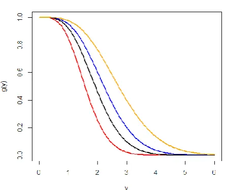
object on the line equals to one. Figure 1 shows the shapes
of the detection function for certain values of 𝜎2. Moreover,
𝑓(𝑦; 𝜎2) is continuous function and proportional to the
𝑔(𝑦; 𝜎2), 𝑓(𝑦; 𝜎2) is decreasing function and related with
𝑔(𝑦; 𝜎2) as
𝑔(𝑦; 𝜎2) = 𝜇𝑓(𝑦; 𝜎2), (13)
where
𝜇 = ∫ 𝑔(𝑦; 𝜎∞ 2)𝑑𝑦
0 . (14)
Then, the corresponding pdf of 𝑔(𝑦; 𝜎2), given by Saeed et
al., (2017) as
𝑔(𝑦; 𝜎2) = 𝑓(𝑦; 𝜎2)(2 − 𝑒−𝑦2⁄2𝜎2
)𝑒−𝑦2⁄2𝜎2
; 𝑦 ≥ 0 , 𝜎2> 0
(15)
By solving the integration in equation (14), the 𝑓(0; 𝜎2) is
given as (Saeed et al., 2017)
𝑓(0; 𝜎2) = 2
(2√2−1)√𝜋𝜎2 (16)
Equation (16) shows that the 𝑓(0; 𝜎2) is a function with the
parameter 𝜎2. Therefore, it is enough to estimate 𝜎2 for
estimating 𝑓(0; 𝜎2) . The considered model in equation (15)
was studied by Noryanti et al. (2018), the maximum
likelihood (MLE) method is used to estimate the proposed
estimator, the performance of the proposed estimator is
evaluated by simulation study. In next section, for this
purpose, kernel method with the proposed model are used to compute the smoothing parameter and studied the
Figure 1. The detection function 𝑔(𝑦) graph of the proposed
model for different parameter 𝜎2
III. KERNAL ESTIMATORR
Consider 𝑌1,…,𝑌𝑛 be random sample of size 𝑛, distributed from
continuous probability density function (pdf) 𝑓(𝑦). According
to in Silverman (1986) and (2018), the kernel estimate 𝑓̂(𝑦) of
𝑓(𝑦) supported on [0; ∞), is given by
𝑓̂(𝑥) = 1
𝑛ℎ∑ (𝐾 ( 𝑦−𝑌𝑖 ℎ ) + 𝐾 (( 𝑦+𝑌𝑖 ℎ ))) 𝑛
𝑖=1 ; 𝑦 ≥ 0 , (17)
where ℎ is the bandwidth, which controls the smoothness of the
fitted function shape and 𝐾 is a kernel function, assumes to be
symmetric function and satisfies the following
∫−∞∞ 𝐾(𝑡)𝑑𝑡 = 1, ∫−∞∞ 𝑡𝐾(𝑡)𝑑𝑡 = 0, ∫∞ 𝑡2𝐾(𝑡)𝑑𝑡 = 𝑐
−∞ ≠ 0 .
(18)
the standard kernel estimate 𝑓̂(0) of 𝑓(0) is given by Chen
(1996) as,
𝑓̂(0) = 2
𝑛ℎ∑ 𝐾 (
𝑌𝑖 ℎ) 𝑛
𝑖=1 . (19)
By assuming 𝑛ℎ → ∞ as 𝑛 → ∞, the bias and variance of 𝑓̂𝑘(0)
can be represented as
𝐵𝑖𝑎𝑠 (𝑓̂𝑘(0)) = 2ℎ𝑓′(0) ∫ 𝑢𝑘(𝑢)𝑑𝑢 ∞
0 +
ℎ2𝑓′′(0) ∫ 𝑢∞ 2𝑘(𝑢)𝑑𝑢 + 𝑜(ℎ2)
0 (20)
and
𝑉𝑎𝑟 (𝑓̂𝑘(0)) = 4𝑓(0)
𝑛ℎ ∫ 𝐾
2(𝑢)𝑑𝑢 ∞
0 + 𝑜(𝑛
−1 ℎ−1 ) (21)
Depending on the assumption that the shoulder condition is true, and the function 𝑓(0) has continuous derivative. Thus, lead us to introduce the following estimator.
𝑓(0) = 𝑓̂𝑘(0) − ℎ2 𝑓′′(0) ∫ 𝑢2𝐾(𝑢)𝑑𝑢 ∞
0 . (22)
The 𝑓′′(0) is the second derivative of 𝑓(𝑦) at 𝑦 = 0. Based
on equation (22) and for underlying 𝑓(𝑦) which satisfies
the shoulder condition, the bias of 𝑓̂(0) is given as
𝐵𝑖𝑎𝑠 (𝑓̂(0)) =2ℎ3𝑓6(3)(0)∫ 𝑢∞ 3𝐾(𝑢)𝑑𝑢
0 +
2ℎ4𝑓(4)(0)
24 ∫ 𝑢
4𝐾(𝑢)𝑑𝑢 ∞
0 + 𝑂(ℎ5) . (23)
and the variance of 𝑓̂(0) is
𝑉𝑎𝑟 (𝑓̂(0)) = 4
𝑛ℎ𝑓(0) ∫ (𝐾(𝑢))
2
𝑑𝑢
∞
0 + 𝑜(𝑛−1 )
(24)
From equations (23), (24) and the assumption that
𝑓′(0) = 𝑓′′′(0) = 0 ,
the asymptotic mean square error (AMSE) can be written as
𝐴𝑀𝑆𝐸 ( 𝑓̂(0)) = 4
𝑛ℎ𝑓(0) ∫ (𝐾(𝑢))
2 𝑑𝑢 ∞ 0 + 2ℎ8 576(𝑓
(4)(0) ∫ 𝑢∞ 4𝐾(𝑢)𝑑𝑢
0 )
2
(25)
The key aspect in nonparametric kernel method the value
ℎ which plays the major milestone in the performance of
𝑓̂𝑘(0). A large smoothing parameter ℎ leads to an estimate
with small variance and large bias while a small h produces a large variance and small bias. Then, the minimisation of the AMSE in equation (25) leads to compute the optimal value of ℎ, which is given by
ℎ = ( 72𝑓(0) ∫ (𝐾(𝑢))
𝟐 𝑑𝑢 ∞
0
(𝑓(4)(0) ∫ 𝑢∞ 4𝐾(𝑢)𝑑𝑢
𝟎 )
𝟐) 1 9⁄
𝑛−1 9⁄ . (26)
The smoothing parameter h in equation (26) depends on
𝑓(0) , 𝑓(4)(0) and the kernel function 𝐾(𝑢). The negative
exponential, half normal models and the proposed model in equation (15) are used as references to compute the smoothing parameter ℎ. In this paper for all models, we use standard normal 𝑁(0; 1) as a kernel function. The optimal values ℎ for the different estimators have been
0.949713𝑇𝑛−1 9⁄ for 𝑓̂
2;𝑘(0) and ℎ3 = 0: 904949𝑌̅𝑛−1 9⁄ for
the proposed estimator 𝑓̂3;𝑘(0), respectively, where 𝑌̅ is
sample mean and 𝑇 = √1
𝑛∑ 𝑦𝑖
2 𝑛
𝑖=1 .
IV. SIMULATION RESULT AND DISCUSSION
A simulation study is performed in order to investigate the
performances of the considered estimators in Section 3. The
data is simulated using one of commonly models used in line
transect which is Hazard-Rate (HR) model (Hemingway (1971) given as
𝑓(𝑥) =𝛤(1−1 𝛽)1⁄ (1 − 𝑒−𝑥−𝛽
) , 𝑥 ≥ 0 , 𝛽 ≥ 1. (27)
For this purpose, we used HR model to generate 400
samples of sizes 𝑛 = 50, 100 and 𝑛 = 200 of
perpendicular distances data set. Four HR models is
selected with parameter values 𝛽 and the corresponding
truncated value 𝑤 are given as (𝛽; 𝑤) =
{(1.5, 20), (2, 12), (2.5, 8); (3, 6)}. The Relative Mean Error (RME) and Relative Bias (RB) be estimated to evaluate the
performance of the estimators 𝑓̂1;𝑘(0), 𝑓̂2;𝑘(0), and 𝑓̂1;𝑘(0).
The RME and RB is given by
𝑅𝑀𝐸 =√𝑀𝑆𝐸(𝑓̂(0))
𝑓(0) , (28)
and
𝑅𝐵 =𝐸(𝑓̂(0))−𝑓(0)
𝑓(0) . (29)
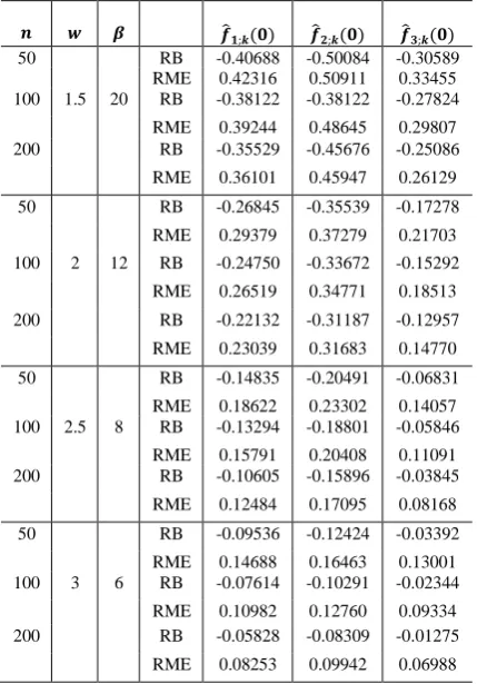
The results of RME and RB are summarised in Table 1.
Table 1. Simulated values of RB and RME for the different estimators.
Table 1 shows that the results of RB and RME in of the three
considered estimators which demonstrated in Section 3. The
estimator 𝑓̂1;𝑘(0) is performed better than 𝑓̂2;𝑘(0) for all
considered cases regardless of sample size n. For each sample
size and for all considered cases, the estimator 𝑓̂1;𝑘(0)
provides the smallest value of RME and RB comparing to
the estimators 𝑓̂1;𝑘(0)and 𝑓̂1;𝑘(0). Indeed, the significant
result is that the performance of proposed estimator
𝑓̂3;𝑘(0)is outperformed well-known considered estimators.
𝒏 𝒘 𝜷 𝒇̂𝟏;𝒌(𝟎) 𝒇̂𝟐;𝒌(𝟎) 𝒇̂𝟑;𝒌(𝟎)
50 RB -0.40688 -0.50084 -0.30589
RME 0.42316 0.50911 0.33455 100 1.5 20 RB -0.38122 -0.38122 -0.27824
RME 0.39244 0.48645 0.29807
200 RB -0.35529 -0.45676 -0.25086
RME 0.36101 0.45947 0.26129
50 RB -0.26845 -0.35539 -0.17278
RME 0.29379 0.37279 0.21703
100 2 12 RB -0.24750 -0.33672 -0.15292
RME 0.26519 0.34771 0.18513
200 RB -0.22132 -0.31187 -0.12957
RME 0.23039 0.31683 0.14770
50 RB -0.14835 -0.20491 -0.06831
RME 0.18622 0.23302 0.14057 100 2.5 8 RB -0.13294 -0.18801 -0.05846
RME 0.15791 0.20408 0.11091
200 RB -0.10605 -0.15896 -0.03845
RME 0.12484 0.17095 0.08168
50 RB -0.09536 -0.12424 -0.03392
RME 0.14688 0.16463 0.13001
100 3 6 RB -0.07614 -0.10291 -0.02344
RME 0.10982 0.12760 0.09334
200 RB -0.05828 -0.08309 -0.01275
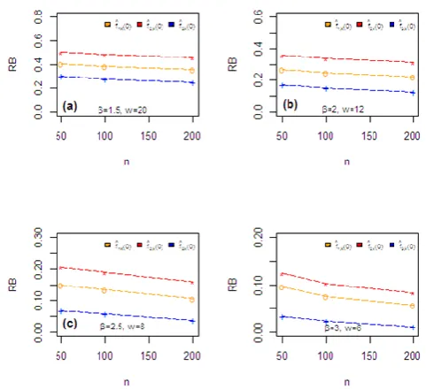
Another noticeable results, the values of RME decrease as the
sample size increases for all estimators which indicates that
the consistency of the proposed estimators for 𝑓(0). This
result can be shown in Figures 2 and 3.
Figure 2. RME values for the different estimators
V. CONCLUSION
In this paper, parametric model is used to construct the
nonparametric kernel estimator 𝑓(0). Moreover, the
smoothing parameter of the kernel estimator is computed for
considered estimators, which plays a major milestone in the
performance of the kernel estimator. Simulation study is
constructed to compare the performance of the proposed
estimator with other existing estimators. The simulated
results of RB and RME indicate that the proposed estimator
is performed better than other estimators considered. In
general, the proposed model be recommended to estimate
𝑓(0) and then to estimate the population density 𝐷.
VI. ACKNOWLEDGEMENT
We gratefully thanks to Universiti Malaysia Pahang for
financial support under Doctoral Research Scheme (DRS)
and RDU170359. We also thanks Ministry of Yemen Higher
Education for sponsor this research study.
VII. REFEREENCES
Buckland, S. T., Anderson, D. R., Burnham, K. P. and Laake, J. L. (1993). Distance sampling. Chapman and Hall, London. Buckland, S. T., Anderson, D. R.,Burnham, K. P., Laake, J. L.
Borchers, D.L., and Thomas, L. (2001). Introduction to distance sampling. Oxford university Press,Oxford.
Buckland, S. T., Rexstad, E. A., Marques, T. A. and Oedekoven, C. S. (2015), Distance sampling: methods and applications, Springer.
Burnham, K. P., Anderson, D. R. (1976).Mathematical models for nonparametric influences from line transect data.Biometrics, 32, 325-336.
Burnham, K. P., Anderson, D. R. and Laake, J. L. (1980). Estimation of density from line transect sampling of biological populations. Wildlife Monograph,72,1-202. Chen, S. X. (1996). A kernel estimate for the density of a
biological population by using line transect sampling. Applied Statistics, pages 135150.
Gates, C, E., Mashall, W. H. and Olson, D. P. (1968). Line transect method of estimating grouse population densities. Biometrics, 24, 135-145.
Hayes, R. J. and Buckland, S. T. (1983). Radial distance models of line transect method. Biometrics, 39,29-42.
Hemingway, P. (1971). Field trials of the line transect method of sampling large populations of herbivores. pp 405-411. The scientific management of animal and plant communities for conservation. Blackwell Sci.
Publ. Oxford.
Noryanti Muhammad, Gamil.A.A.Saeed and Wan Nur Syahidah binti Wan Yusoff, Performance of Parametric Model for Line Transect Data, ASM Sci. J.Special Issue 2018(1).
Saeed, G. A. A., Muhammad, N., Liang, C. Z., Yusoff, W. N. S. W. and Salleh, M. Z. (2017), Model for estimating of population abundance using line transect sampling, in
‘Journal of Physics: Conference Series’, Vol. 890, IOP
Publishing, p. 012153. 85.
Silverman, B. W. (1986). Density estimation for statistics and data analysis.Chapman and Hall, London.