Simulation and real time processing techniques for space instrumentation

(1)

Simulation and Real Time Processing

Techniques

for Space Instrumentation

Hong Joon CHUN

Submitted to the University of London

for the degree of Doctor of Philosophy

December, 1996

Mullard Space Science Laboratory Department of Space and Climate Physics

University College London Holmbury St. Mary

(2)

ProQuest Number: 10045713

INFORMATION TO ALL USERS

The quality of this reproduction is dependent upon the quality of the copy submitted.

In the unlikely event that the author did not send a complete manuscript and there are missing pages, these will be noted. Also, if material had to be removed,

a note will indicate the deletion.

uest.

ProQuest 10045713

Published by ProQuest LLC(2016). Copyright of the Dissertation is held by the Author.

This work is protected against unauthorized copying under Title 17, United States Code. Microform Edition © ProQuest LLC.

ProQuest LLC

789 East Eisenhower Parkway P.O. Box 1346

(3)

Abstract

Designing and developing space instruments involves a wide variety of evaluation and simulation techniques in order to ensure correct operation under all possible conditions likely to be encountered in space and to allow parallel development of different subsystems of an instrument.

This thesis describes three such evaluation and simulation techniques including real-time processing techniques, devised for two major European space missions, the Solar and Heliospheric Observatory (SOHO) and the X-ray Multi-Mirror (XMM) mission.

The design of a Science Data Display Adapter is described, which was developed to provide comprehensive performance evaluation of the detectors of the Grazing Incidence Spectrometer (GIS), part of the Coronal Diagnostic Spectrometer on-board the SOHO, in the absence of the Command and Data Handling System and the Experiment Ground Support Equipment. The requirements to handle high data rates and to have significant display flexibility are discussed.

This thesis also describes a user-controlled detector simulator developed to carry out full range tests of the GIS processing electronics in the absence of real detectors, including extreme conditions not easily achievable by other means. With its large degree of flexibility, the simulator provides realistic shapes and a wide range of characteristics for the output events of the Spiral Anode (SPAN). Although the simulator was designed specifically to simulate the SPAN, the design is applicable to any three channel detector system and has since been used for the FONEMA instrument for the Russian Mars96 mission.

(4)

To God,

who gave me strength, wisdom, peace and comfort

(5)

David said to the Philistine, “You come against me with sword and spear and javelin, but I come against you in the name o f the L O R D Almighty, the God o f the armies o f Israel, whom you have defied. ”

1 Samuel 17:45

Therefore, as G od’s chosen people, holy and dearly loved, clothe yourselves with compassion, kindness, humility, gentleness and patience.

Bear with each other and forgive whatever grievances you may have against one another. Forgive as the Lord forgave you.

And over all these virtues pu t on love, which binds them all together in perfect unity. Let the peace o f Christ rule in your hearts, since as members o f one body you were called to peace. A nd be thankful.

Let the word o f Christ dwell in you richly as you teach and admonish one another with all wisdom, and as you sing psalms, hymns and spiritual songs with gratitude in your hearts to God.

A nd whatever you do, whether in word or deed, do it all in the name o f the Lord Jesus, giving thanks to God the Father through him.

(6)

Table o f Contents

ABSTRACT... 2

TABLE OF CONTENTS... 5

LIST OF FIGURES... 10

LIST OF TABLES... 15

CHAPTER 1. GENERAL INTRODUCTION... 16

CHAPTER 2. SOLAR AND HELIOSPHERIC OBSERVATORY... 19

2.1 Mission History and Background...19

2.2 The Solar Wind Acceleration and the Heating of the C o ron a...21

2.3 The SOHO M ission... 22

2.3.1 Scientific Goals o f SO H O...22

2.3.2 Measurements Required to Accomplish the Goals... 22

2.3.3 Payloads...23

2.3.3.1 Coronal Instrum ents... 23

2.3.3.2 Helioseismology Instruments...24

2.3.3.3 Solar Wind “In-Situ” Instrum ents...26

2.3.4 Other Roles o f SO H O...27

2.3.5 Mission D esign... 27

2.3.5.1 Spacecraft... 27

2.3.5.2 O rbit... 29

2.4 The Coronal Diagnostic Spectrometer... 30

(7)

Table of Contents 6

CHAPTER 3. SCIENCE DATA DISPLAY ADAPTER...35

3.1 Introduction... 35

3.2 Operation of the G IS... 37

3.2.1 GIS Analogue Electronics...40

3.2.2 Science Data Stream...42

3.2.2.1 Look Up Table...43

3.2.2.2 First In First Out B uffer...43

3.2.2.3 Other Conversions...44

3.2.3 GIS Simulator...44

3.3 SDDA Specifications and Requirem ents... 45

3.3.1 Interface with the GIS...45

3.3.2 SDDA Performance Requirements...45

3.4 SDDA Hardware Description...48

3.4.1 Use o f Differential Amplifiers...49

3.4.2 Transferring D a ta...50

3.4.2.1 Address M ap... 54

3.4.2.2 Address Decoding M ethod...55

3.4.2.3 Activating the 16-bit Data B u s...57

3.4.3 Data Conversion and Acquisition...58

3.4.3.1 Setup and Hold Time Requirements...62

3.4.4 Timer...64

3.4.4.1 General Functional Description of the P IT ...65

3.4.4.2 Configuration of the P IT ...66

3.4.4.3 External Clock Generation... 68

3.4.4.4 Usage of the Counters in the PIT... 68

3.4.5 Control L ogic...68

3.4.5.1 Function and Configuration of the P P I... 69

3.4.5.2 Data Acquisition at Different Count Rates...72

3.4.5.3 Dealing with Unused Inputs... 73

3.5 SDDA Software D escription...73

3.5.1 Controlling and Programming...74

3.5.2 User Interface...74

(8)

3.6 Results and D iscussion... 83

5.6.1 Future Work on Performance Im provem ent...83

3.6.2 Results...83

CHAPTER 4. MICROCHANNEL PLATE BASED SPIRAL ANODE DETECTOR SIMULATION...89

4.2 SPAN R eadouts...93

4.2.1 Widths o f the SPAN Electrodes...93

4.2.2 SPAN P ositions...98

4.3 Effects of the MCP on the SPAN Perform ance... 99

4.3.1 Charge Cloud Distribution and Sym m etry... 99

4.3.2 Modulation and Convolution E ffec ts...100

4.3.3 Effects o f MCP Operating Parameters on Charge Cloud Size...102

4.3.4 Gain Depression...103

4.3.4.1 Gain Depression at High Output Count Rates... 103

4.3.4.2 Gain Fatigue... 104

4.3.5 Modelling the M C P...105

4.4 DetSim Design Specifications and Properties... 105

4.4.1 DetSim Properties and Specifications...107

4.4.2 Time Intervals between Successive P hotons...110

4.5 DetSim Software...111

4.5.1. User Interfa ce...112

4.5.2. Software Configuration...116

4.5.3. Random Number Generation...119

4.5.4 SPAN Position G eneration...121

4.5.5. Data Calibration and S/W Verification...122

4.6 Digital Hardware...123

4.6.1 Address Decoding and Data Transfer...123

4.6.2 Data Storage...124

4.6.3 PC-lnterface...127

(9)

4.6.5 Timer and External Clock...129

4.6.6 Simulation Process Description...130

4.7 Analogue H ardw are...134

4.8 Board Lay o u t... 138

4.9 Results and D iscussion... 138

CHAPTER 5. X-RAY MULTI-MIRROR MISSION... 146

5.2 The XMM Spacecraft... 150

5.2.1 The EPIC Instrument...152

5.2.2 The OM Instrum ent...152

5.2.3 The RGS Instrum ent...153

5.3 Functional Description of the R G S ...156

5.3.1 CCD Read-out...156

5.3.2 The RGS Operating M odes...157

5.3.3 The RGS Analogue Electronics...158

5.3.4 The RGS Digital Electronics...158

5.3.5 Data Pre-Processor...159

CHAPTER 6. ON-BOARD EVENT PROCESSING ALGORITHMS...162

6.2 Events from RGS C CD s...165

6.2.1 Pile-up C riterion...165

6.2.2 Event Categories...166

6.2.3 Event M orphology...166

6.3 Event Processing Requirements for the D PP...170

6.4 Event Processing Algorithms... 172

6.4.1 Event Processing Algorithm 1 (EPA I )...173

6.4.2 Event Processing Algorithm 11 (EPA II)...179

6.5 Experiments and Test Set-U p...186

6.5.1 Implementation Language, Ada versus Assem bly...186

(10)

6.5.3 EOBB DPP Test Set-u p...188

6.6 Concept of Handling Cosmic Ray Events...193

6.7 Experimental Results and Discussion... 195

CHAPTER 7. CONCLUSIONS... 203

BIBLIOGRAPHY... 206

(11)

List o f Figures

Chapter 2

2.1 SOHO spacecraft schematic view ...24

2.2 Wavelength and temperature coverage of the four UV coronal instruments SUMER, CDS, UVCS and BIT with some selected emission lines... ... 26

2.3 The SOHO spacecraft consists of two independent elements, the Payload Module (PLM) and the Service Module (SV M )...28

2.4 SOHO O rbit...29

2.5 The Optical Layout of the CDS with the GIS Processing Electronics...31

2.6 Solar spectra of the quiet Sun from the GIS detectors... 34

Chapter 3

3.1 (a) Actual flight development system, (b) SDDA ‘simulates’ CDHS and E G S E ... 36

3.2 Diagram showing the path from a photon to its spectrum... 38

3.3 Principle of operation of the G IS ... 39

3.4 A 1-D SPAN anode... 40

3.5 GIS Analogue Electronics...41

(12)

List of Figures 11

3.6 Schematic diagram of the data flow in the Science Data Processor...42

3.7 Data format from the GIS... 44

3.8 Timing diagrams of the interface signals at various event rates... 46

3.9 Block diagram of the SDDA...49

3.10 Circuit diagram of the SDDA hardw are... 51

3.11 I/O cycles... 53

3.12 I/O addresses for IBM P C ... 54

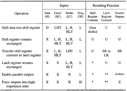
3.13 Block diagram of the Serial-Input/Serial- or Parallel-Output Shift Register (74H C 595)...59

3.14 Data bus... 60

3.15 Timing diagram of the input/output d ata... 61

3.16 Timing requirements of the H C595... 64

3.17 Control Word format... 67

3.18 Extended stro b e... 72

3.19 SDDA screen... 75

3.20 Examples of SDDA display screens in input m o d e... 78

3.21 Examples of SDDA display screens showing three accumulation modes... 80

3.22 Flow diagram of data acquisition...82

3.23 Flow diagram of data acquisition with a Check_Flag...84

3.24 SDDA display of data taken from the G IS_S IM ...87

3.25 Data spectrum taken from a Thermal/Vacuum test of the GIS, using the SDDA ....88

Chapter 4

4.1 Test configuration for the GIS Processing Electronics (G P E )... 90

4.2 Schematic diagram o f the SPAN, showing the widths (w%, Wy and w j of the electrodes (X, Y and Z) (not to scale)...94

4.3 The locus representing the variation of the electrodes along the anode plotted in the 3-D volume defined by the fractional charges on the electrodes...95

4.4 The evolution of the spiral as the photon position varies along the anode... 96

(13)

4.6 Spiral arms in r - 0 coordinates... 98

4.7 Effects of modulation and convolution... 101

4.8 Gain depression with increasing count ra te ... 104

4.9 DetSim system test setup diagram ...106

4.10 Plot showing the simple exponential shape describing the time intervals between successive ev en ts...I l l 4.11 Examples of a user interface screen ... 114

4.12 Block diagram of the DetSim hardw are... 117

4.13 Schematic flow diagram of the simulation p ro cess... 118

4.14 Shuffling procedure used in ran i to break up sequential correlations in the Minimal Standard generator... 120

4.15 Transformation method for generating a random deviate y from a known probability distribution p ( y )... 121

4.16 Conceptual circuit diagram of the DetSim D H ... 126

4.17 Simplified diagram showing the start, stop and synchronization m ethods...128

4.18 Timing diagram of the control and synchronized pulses... 129

4.19 Timing diagram of the data transfer... 131

4.20 Circuit diagram of the GIS DetSim Analogue H ardw are... 135

4.21 GIS pulse shaping schem e... 136

4.22 GIS DetSim grounding scheme... 137

4.23 SOHO-CDS GIS Detector Simulator b o x ... 139

4.24 DetSim flat field outp ut...141

4.25 Spiral images...142

4.26 DetSim output image at a fixed position... 144

Chapter 5

5.1 Overview of the XMM spacecraft...147

(14)

5.3 Exploded view of the spacecraft configuration showing the service and payload

m odules... 150

5.4 Layout of the three XMM instruments... 151

5.5 Spectral resolving power of a single module RGS as a function of wavelength 154 5.6 The effective area of the RGS (single module) in first and second order as a function of w avelength... 154

5.7 Schematic showing the operating principle of the R G S ...155

5.8 Schematic layout o f the RG S... 155

5.9 XMM RGS electrical sub-system s... 156

5.10 DPP single processor functional layout...160

Chapter 6

6.1 Event categories...167

6.2 Examples of some of possible patterns of split events caused by genuine X-rays .... 168

6.3 Example of event shapes on a C C D ...169

6.4 Input buffer stru ctu re...172

6.5 Top level flow diagram of EPA 1... 174

6.6 Flow diagram of the FORWARD subroutine for EPA I ...175

6.7 Flow diagram of the BACKWARD subroutine for EPA 1 ... 176

6.8 Flow diagram o f the RECONSTRUCTION subroutine for EPA 1... 177

6.9 Top level flow diagram of EPA II... 180

6.10 Flow diagram of the SEARCH subroutine for EPA I I ...181

6.11 Flow diagram of the RECONSTRUCTION subroutine for EPA I I ... 182

6.12 Flow diagram of the FORWARD subroutine for EPA I I ... 183

6.13 Flow diagram of the BACKWARD subroutine for EPA I I ...184

6.14 Example of performance test of EPA I with some of the patterns in Figures 6.2 and 6.3 using the verification tool...189

6.15 Example of performance test of EPA II with some of the patterns in Figures 6.2 and 6.3 using the verification tool...190

(15)

6.17 Oscilloscope display in measuring the speed of the E P A s... 192

6.18 Example of a case of algorithm failure...195

6.19 Patterns where 50 % of events are split ( 1 x 1 on-chip binning)...196

6.20 Patterns where about 17 % of events are split ( 3 x 3 on-chip binning)... 196

6.21 Single events...197

6.22 Cosmic ray ev en ts...198

(16)

List o f Tables

Chapter 2

2.1 The SOHO scientific instrument payload... 25

Chapter 3

3.1 Port addresses used in the S D D A ... 55

3.2 Summary of the I/O operation of the GIS data...63

3.3 Operations of the P IT ...66

3.4 Operations of the P P I...70

3.5 Mode 0 Port configurations... 71

3.6 SDDA commands and operations... 76

Chapter 4

4.1 Options available in the D S/W ... 115

4.2 Port addresses used in the D etSim ... 125

Chapter 6

6.1 Number of pixels EPA I and II can process per second for the event patterns in Figures 6.19 - 6.23 for a MA31750 processor running at 4 M H z... 200

(17)

C H A P T E R

1

"The end o f all things is near. Therefore be clear m inded and self-controlled so that you can pray.

Above all, love each other deeply, because love covers over a m ultitude o f sins.

Offer hospitality to one another without grumbling.

Each one should use whatever g ift he has received to serve others, faithfully administering G o d ’s grace in its various form s.

I f anyone speaks, he should do it as one speaking the very words o f God. I f anyone serves, he should do it with the strength God provides, so that in all things G od m ay be praised through Jesus Christ. To him be the glory and the po w er fo r ever and ever. Amen. ”

1 P eter 4 :7 -1 1

General Introduction

It is absolutely vital to ensure that scientific space instruments will operate successfully under all possible conditions likely to be experienced during actual space missions. Applications of modem simulation techniques involving computers, hardware electronics and software to space instmmentation can provide quick and versatile equipment which can be used to test and to validate actual flight space instruments, prior to its use in space, for a wide variety of conditions, including extremes, which are likely to be encountered in space.

In developing and testing space instruments, it is also very important to simulate various subsystems of an instrument to allow testing and calibrating the subsystems independently without necessarily having all the flight pieces of equipment available in the same place at the same time. This thus makes parallel development of different parts of the instmment possible.

(18)

Chapter 1. General Introduction 17

The versatility of the simulation and test equipment can be of great assistance in detecting, understanding and solving any problem which might arise in the integrated system long before the actual integration of the whole instrument takes place, as well as in confirming the subsystem design.

In general, a scientific space instrument can be considered to consist mainly of three subsystems: a detector sensor which collects raw scientific data and converts them to electrical signals - it may consist of some form of electron multiplier, such as MicroChannel plates, and an anode, such as the Spiral Anode (SPAN, see Chapter 4), the wedge and strip anode, delay lines and Charge Coupled Devices (CCDs); detector electronics which converts the electrical signal from a sensor into meaningful scientific data; and control electronics to supply power, to control and monitor the whole instrument, to collect scientific and engineering data and to provide a telemetry link with the spacecraft. In addition, an Experiment Ground Support Equipment (EGSE), which is not part of the instrument, is generally required to aid development and testing of the instrument.

This thesis describes three different aspects of simulation techniques, including real-time processing techniques, involving two major European space missions that form part of the

European Space Agency’s Horizon 2000 program: the Solar and Heliospheric

(19)

Chapter 1. General Introduction 18

events split over two or more adjacent pixels, and to study the feasibility of having a single processor Data Pre-Processor (DPP) in the RGS Digital Electronics to handle all incoming event data. Two on-board X-ray event processing algorithms were developed and used to validate the design of the single processor DPP: the performance of the DPP was tested using both algorithms with several different kinds of event patterns that are likely to be formed by X-rays and background cosmic rays during the course of the XMM mission. Since one of the two algorithms described in this thesis will actually be used for flight, the algorithms themselves needed to be tested under all possible predictable conditions, and a way of validating the algorithms by simulating their CCD data input is also discussed.

(20)

C H A P T E R

“Trust in the Lord with all you heart and lean not on your own understanding;

in all your ways acknowledge him, and he will m ake your paths straight.

Do not be wise in your own eyes; fe a r the Lordand shun evil. ”

Proverbs 3 :5 -7 “Commit to the LORD whatever you do, and your plans will succeed.

In his heart a man plans his course, but the LO RD determ ines his steps.

B etter a patient man that a warrior, a man who controls his tem per than one who takes a city. ”

Proverbs 6:3, 9, 32 “A m a n ’s pride brings him low, but a man o f lowly spirit gains honor. ”

Proverbs 29:23

Solar and Heliospheric Observatory

The Solar and Heliospheric Observatory (SOHO) is a space mission flown as part of the Solar Terrestrial Science Programme (STS?) which is carried out collaboratively by the European Space Agency (ESA) and the National Aeronautics and Space Administration (NASA). The SOHO constitutes the first ‘cornerstone’ of ESA ’s scientific long-term programme, "Space Science-Horizon 2000’.

2.1 MISSION HISTORY AND BACKGROUND

Solar coronal studies were very much limited to brief views (Domingo et al., 1995) during solar eclipses until ultraviolet observations of the Sun were made from space using rocket

(21)

Chapter 2. Solar and Heliospheric Observatory 20

experiments by Baum et a l (1946). Shortly after that, NASA launched a series of Orbiting Solar Observatory (OSO) missions (Athay and White, 1978) to observe the Sun in the ultraviolet (UV) and X-ray region of the spectrum. Although these observations were made with what today would be described as relatively primitive spacecraft and telescopes, they showed much could be learned about the Sun by studying it using space- based telescopes.

The Apollo Telescope Mount (ATM) (Tousey, 1977), the most sophisticated complement of solar telescopes to operate in space to date, was flown on Skylab (Withbroe and Noyes, 1977; Vaiana and Rosner, 1978) and provided high resolution X-ray and extreme ultraviolet (EUV) images of the Sun, high resolution UV spectra of the chromosphere and corona and high resolution white light images of the outer electron corona. Since most of the observations were made with photographic film or photomultipliers, only a limited amount of data could be recorded, providing a very restricting temporal resolution (Domingo et a l, 1995). Skylab also clearly showed that future observations would need to have high spatial resolution, high time resolution, wide spectral coverage and extended observing time scales.

After Skylab, the Solar Maximum Mission (SMM) was flown to study solar flares (Bohlin

et a l , 1980), using high energy X-ray detectors, a UV spectrograph and a white light coronagraph. Although SMM greatly expanded our understanding of solar flares by providing simultaneous observations of flares in the X-ray and UV spectral regions, there was no EUV spectrograph on SMM so the critical temperature range between approximately 0.5 x 10^ K and 1 x 10^ K was not observed (Domingo et a l , 1995). Since detectors that were available at the time SMM was developed did not have the sensitivity and spatial coverage available now, the observations were additionally limited.

(22)

(Christensen-Chapter 2. Solar and Heliospheric Observatory 21

Dalsgaard, 1992; Leibacher, 1995) was included as one of the goals of SOHO (Domingo, 1988) when it became clear that ESA’s DISCO mission, which would have featured the first helioseismology measurements from a spacecraft, was not being implemented.

CLUSTER, a fleet of four satellites taking three-dimensional measurements of the Earth magnetosphere (see also Credland, 1995; Mecke, 1995; Ellwood et a l , 1995; Drigani, 1995; Ferri and Warhaut, 1995 for detail), joined SOHO in the STSP to offer the possibility of a comparative study, by in-situ and remote-sensing observations, of the basic processes of solar-terrestrial physics in the grand context, i.e., on the Sun, in the magnetosphere and in the interplanetary medium. It is hoped that these missions will fill the ‘gaps’ that have not yet been investigated in solar and plasma physics.

2.2 THE SOLAR WIND ACCELERATION AND THE HEATING

OF THE CORONA

Many basic physical processes of the inner corona are inter-related with the physics of the extended corona, the solar wind and the interplanetary medium (Huber and Malinovsky- Arduini, 1992). For example, information on electron and ion densities and temperatures, and on flow velocities as a function of radial distance in the extended corona is important for investigating solar wind acceleration (Kohl and Withbroe, 1982).

Particle acceleration by shock waves is important in understanding heating mechanisms of solar corona because in the case of corona shocks, much of the shock energy is eventually converted to thermal energy and thus may be a significant contributor to coronal heating (Huber and Malinovsky-Arduini, 1992).

(23)

2.3 THE SOHO MISSION

2.3.1 Scientific Goals o f SOHO

SOHO will address the following three fundamental, yet still enigmatic questions of solar physics:

• What is the structure and dynamics of the Sun’s interior? (helioseismology)

• How is the Sun’s corona formed and heated? (remote sensing)

• Where and how are the solar wind streams accelerated? (in-situ)

These scientific goals of SOHO match the status of solar physics following the results of previous space missions, and reflect the state of the art in instrument technology and spacecraft and mission design although there is also a cost aspect to be considered.

2.3.2 Measurements Required to Accomplish the Goals

The study of the high temperature coronal plasma is best carried out at EUV and soft X- ray (XUV) wavelengths where the strongest emission lines of relevant highly ionized atoms are located. According to Huber and Malinovsky-Arduini (1992), a reliable test of the models of coronal and solar-wind structures and processes requires precise measurements of critical parameters in the relevant components which necessitates sufficiently well-calibrated instruments for remote-sensing observations as well as in-situ

measurements on SOHO.

For the lower corona, the critical parameters are obtained by simultaneous observations of chromospheric, transition-zone and coronal plasma by recording emission lines between 170 and 1600 A, whereas for the higher parts of the corona, where the solar wind is believed to be accelerated, coronographic techniques combined with spectroscopic measurements must be used (Huber and Malinovsky-Arduini, 1992).

(24)

a spatial resolution of about 1 arc sec in order to resolve the fine structure of the inner corona,

a spectral resolution o f about 5x10"^ with sufficient signal-to noise ratio, to record line profiles and to determine line-of-sight velocities from Doppler shifts with an accuracy of the order of 1 km/s,

• a time resolution of the order of 10 sec. to follow dynamically evolving features like jets and bright points.

To determine the radial stratification of the Sun, oscillation-mode frequencies of

p-(standing acoustic waves) and all available g-modes p-(standing internal gravity waves) (Christensen-Dalsgaard, 1992) are required in principle. Inversion of the mode-frequency data then would yield the stratification of pressure and density, which in turn can be used to test our understanding of the physics of the dense plasma which constitutes the solar interior.

2.3.3 Payloads

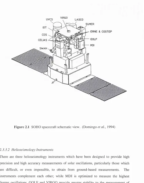
To achieve the scientific goals of the mission, SOHO carries a payload consisting of 12 sets of complementary instruments (see Figure 2.1): six atmospheric (coronal) remote sensing, three helioseismology and three solar wind particle in-situ instruments. Their characteristics are briefly summarized in Table 2.1.

2.3.3.1 Coronal Instruments

(25)

UVCS VIRGO

SUMER

ERNE & COSTEP

GOLF CELIAS

SWAN

Figure 2.1 SOHO spacecraft schematic view. (Domingo e ra /., 1994)

2.33.2 Helioseismology Instruments

(26)

Investigation Measurements Technique References (see also)

SO L A R A TM O SPH ER E R EM O TE SEN SIN G

SUMER Plasma flow characteristics

(Temperature, density, velocity)

chromosphere through corona

Normal incidence spectrometer,

500-1600Â , spectral res.

20000-40000, angular res. = 1.3"

(Wilhelm era/., 1989;

Wilhelm et a i , 1995;

Lemaire and Wilhelm, 1994)

CDS Temperature and density: transition

region and corona

Normal and grazing incidence

spectrometer, 150-800Â, spectr.

res. 1000-10000, angular res. = 3"

(Harrison et a i , 1995;

Kent et a i , 1995;

Harrison and Fludra, 1995)

EIT Evolution of chromospheric and

coronal structures

Full disk images (42'x42' with

1024x1024 pixels) in He II, Fe IX,

Fe XII and Fe XV

(Delaboudinière era/., 1995)

UVCS Electron and ion temperature,

densities, velocities in corona

(1.3-10 R®)

Profiles and/or intensity o f selected

EUV lines (Ly-o, O VI, etc.)

between 1.3 and 10 R@

(Kohl era/., 1995)

LASCO Evolution, mass, momentum and

energy transport in corona

(1.1-30 R®)

I internally and 2 externally

occulted coronagraphs; Fabry-Perot

spectrometer for 1.1-3 R@

(Brueckner era/., 1995)

SWAN Solar wind mass flux anisoptropies

and its temporal variations

Scanning telescopes with hydrogen

absorption cell for L y -a light

(Bertaux era/., 1989;

Bertaux era/., 1995)

H ELIO SEISM O LO G Y

GOLF Global Sun velocity oscillations

(/= 0 -3 )

Na-vapour resonant scattering cell,

Doppler shift and circular

polarization

(Gabriel et a i , 1995)

VIRGO Low degree {£=0-7) irradiance

oscillations and solar constant

Global Sun and low resolution

(12 pixels) imaging, active cavity

radiometers

(Frohlich era/., 1995)

MDI/SOI Velocity oscillations, harmonic

degree up to 4500

Fourier tachometer, angular

resolution: 1.3 and 4"

(Scherrer era/., 1995)

SO LAR W IND ‘IN S IT U ’

CELIAS Energy distribution and

composition (mass, charge,

chargestate) (0.1-1000 keV/e)

Electrostatic deflection,

time-of-flight measurements, solid state

detectors

(Hovestadt era/., 1995)

COSTEP Energy distribution of ions (p. He)

0.04-53 MeV/n and electrons

0.04-5 MeV

Solid state and plastic scintillator

detectors

(Müller-Mellin et a i , 1995)

ERNE Energy distribution and isotopic

composition o f ions (p-Ni) 1.4-540

MeV/n and electrons 5-60 MeV

Solid state and plastic scintillator

detectors

(Torsti et al., 1995;

Lumme era/., 1995)

Table 2.1 The SOHO scientific instrument payload.

(27)

EIT • • • •

1st ...

2 n d ...

NI ... {zzzza

CDS

UVCS ■7773-U7n

Gl V//77A VJJjm Ÿ77777Z2-1st ...

SUMER 2nd 107 10' QJ t_ D O L _ QJ CL E QJ _10'

-]— I— I— I— I— I— I— I— I— 1— I— I— I— I— I I I I I I r

, F . XIX O F« XVIII

.CoXIV .N D M I ,F*XV1

, F . XV«

/ • ^ . X V ,F.XV , s l X , FeXM ,SXI . S » «XI " S ' *

X"' . F . XII . S X . o «F» XI ^ d X .S IK .MglX

,F*VHI

,C o X

M g VIII

N « VIII

,N« IX ,a VIII

. C c V»l . N , VII . M g VI _

. N « VI , N e VI

-. N « V . 0 V 1 W . V . M g V

. 0 V . 0 V • , 0 V

. N * IV , S V 1 « S V 1 . 5 VI

-. 0 N P rv . 0 fv _{. N IV}

, S IV , S i N .S I IV

#H dl

,C IV.

. N n . N i l

.•^y.â^.àV .Lyy

-.1 V *1

200 400 600 800 1000 1200 1400 1600

W a v e l e n g t h [A]

F ig u re 2.2 Wavelength and temperature coverage of the four UV coronal instruments SUM ER, CDS, UVCS and EIT with some selected emission lines. N ote the overlap in wavelength bands of all instruments, important for inter-calibration. (Domingo et aL, 1995).

2.3.3.3 Solar Wind “In-Situ” Instruments

(28)

2.3.4 Other Roles o f SOHO

SOHO will also contribute to the understanding of mass supply and flows in the solar corona. Plasma flows (expected in the regions where energy is released during magnetic reconnection and whenever there is a pressure difference either between the footpoints or between the coronal and chromospheric segments of a coronal loop), such as siphon flows or convective flows of chromospheric material evaporating into the corona, can induce phenomena of spatial and temporal brightness variations of the corona (Antonucci, 1994). In particular, evaporation induces a net mass input into the corona producing consequent coronal density enhancements (Antonucci, 1994). The high spatial, spectral and temporal resolution of the UV spectrometers of SOHO will provide a continuous coverage from the chromosphere to the corona, in the 10^- 10^ K domain (Antonucci, 1994).

Although streamers have been observed since far back in time, a number of problems related to streamer physics and morphology are still unclear. SOHO’s experiments will derive the geometry and 3-D structure of streamers and densities and temperatures in streamers (Poletto, 1994). SOHO will also evaluate element abundances in streamers and

clarify streamer physical conditions including the presence of MHD

(magnetohydrodynamic) waves and the intensity/direction of magnetic fields throughout the streamer body (Poletto, 1994).

Esser (1994) explains how the SOHO instruments can contribute to solving the problems of solar wind expansion by determining the physical processes that are responsible for the behavior of the solar wind plasma and by establishing the physical models that can be used to predict the properties of the plasma flow, or at least certain aspects of it.

2.3.5 Mission Design

2.3.5.1 Spacecraft

(29)

The design of the SOHO spacecraft is based on a modular concept with tw o main elements, the Service M odule (SVM) and the Payload M odule (PLM) (see Figure 2.3). The SVM itself is split into two sub-assemblies: the service equipment module and the propulsion module. This configuration provides easy mounting and accessibility to the payload instruments, while satisfying all instrument functional requirements, particularly viewing direction, field-of-view clearance, straylight avoidance and pointing stability (Bouffard et ai, 1995).

Payload M odule Service M odule

Instruments Attitude Sensors

Propulsion Module

Service Equipment

Module

F ig u re 2.3 The SOHO spacecraft consists of two independent elements, the Payload Module (PLM ) and the Service M odule (SVM). The PLM carries all scientific instruments while house-keeping equipment is mounted onto the SVM. Only the attitude measurement sensors are installed on the PLM for achieving highest alignment stability.

(30)

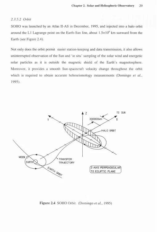
SOHO was launched by an Atlas II-AS in December, 1995, and injected into a halo orbit around the LI Lagrange point on the Earth-Sun line, about 1.5x10^ km sunward from the Earth (see Figure 2.4).

Not only does the orbit permit easier station-keeping and data transmission, it also allows uninterrupted observation of the Sun and ‘in situ’ sampling of the solar wind and energetic solar particles as it is outside the magnetic shield of the Earth’s magnetosphere. M oreover, it provides a smooth Sun-spacecraft velocity change throughout the orbit which is required to obtain accurate helioseismology measurements (Domingo et a l,

1995).

TO SUN

300000km

■HALO ORBIT

MOON

TRANSFER TRAJECTORY

EARTH

'Z-AXIS PERPENDICULAR' JO ECLIPTIC PLANE ,

(31)

2.4 THE CORONAL DIAGNOSTIC SPECTROMETER

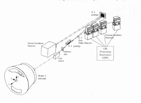
The Coronal Diagnostic Spectrometer (CDS) is one of the coronal instruments on-board the SOHO, which is designed to probe the solar atmosphere through the detection of spectral emission lines in the EUV wavelength range 150 - 800 Â, with spatial resolution better than 3". By observing the intensities and profiles of selected lines, it is possible to derive temperature, density, flow and abundance information for the plasmas in the solar atmosphere (Kent et a l, 1995).

The performance requirements for CDS are as follows (Harrison et a l, 1995):

• Wavelength coverage should include lines from ions formed in the temperature range 10"^ K to a few 10^ K. The region 150 - 800 Â is appropriate for this, the shorter wavelengths being essential for the inclusion of emission lines from the hottest plasmas.

• Spectral resolution should allow separation of the lines of prime interest. Given the crowded nature of the 150 - 220 Â region, although there will inevitably be blend, most lines of prime interest can be separated with a resolution of order ÔA. = 0.3 Â at the shortest wavelengths, where hX is the line width.

• The field of view, without repointing, must be large enough to cover an active region or a large fraction of features such as prominences, coronal holes or of the quiet Sun. If the instrument cannot view the full Sun, re-pointing should allow studies of any region of the disc or low corona.

• Spatial resolution as fine as a few arcseconds must be achieved, appropriate for the smaller scale structures of the solar atmosphere.

• Time resolution should be as short as possible, at least 1 second.

(32)

gratings

G razing W cidence

Detect^

Zero O rder D etector N orm al Incidence

D etector G. I. gratings

G IS Processing Electronics (CPE) entrance

slits

scan m irror

W olter 2 telescope

Figure 2.5 The Optical Layout of the CDS with the GIS Processing Electronics.

(principally Ne, Mg, Si and Fe); well separated, bright lines formed over wide temperature ranges; and several high-temperature lines, e.g. Fe XXI at 270.52 A and Fe XXIII at 263.76 Â (Kent et a l, 1995; see also Harrison et a l (1995) for the list of the lines).

(33)

(Harrison and Fludra, 1995). The two NIS gratings disperse two different wavelength bands, namely 310 - 380 and 520 - 630 Â (Harrison et a l , 1995).

The ideal design for CDS would have been a single NIS system, covering all wavelengths, allowing full advantage of the speed of the NIS system; however, many spectral emission lines produced at the highest temperatures in the quiet solar atmosphere occur at wavelengths much less than 300 Â, and below this value the efficiency of the normal incidence reflection falls dramatically (Harrison and Fludra, 1995).

2.5 GRAZING INCIDENCE SPECTROMETER

All four GIS detectors are identical so as to be fully interchangeable. Their basic requirements to help to achieve the scientific goals of the CDS, discussed above, are as follows (Breeveld and Thomas, 1992):

• positional resolution of 47 pm over a sensitive area of 50 x 16 mm

• quantum efficiency greater than 10%

• event rate of 10^ counts per second

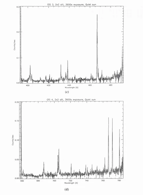
The GIS uses four detector heads, each having a microchannel plate EUV sensor with 1-D position readout. The sensor information is decoded to provide 2048 positions for each detector head which map directly as wavelength. Figure 2.6 shows solar spectrum plots of the quiet Sun* from each detector, obtained with the SOHO-CDS-GIS with a slit size of 2

X 2. This is the GIS prime slit which makes use of the best possible spectral and spatial

characteristics of CDS. However, for lower intensities, one can trade the spectral/spatial information for greater counts with wider slits; the CDS slit selections are listed in Harrison and Fludra (1995).

(34)

Chapter 2. Solar and Heliospheric Observatory 33 GIS 1, 2 x 2 slit, 3 6 0 0 s e x p o s u re, Quiet sun

0.50

0.40

0.30

o

(J

0.20

0 .1 0

0.00

220

200 2 10

170 180 190

160

W o v e le n g th (A)

(a)

CIS 2, 2x 2 slit, 3 6 0 0 s e x p o s u re . Quiet sun 0.15

0 .1 0

o

u

0.05

0.00

300 320

260 280

(35)

Chapter 2. Solar and Heliospheric Observatory 34 GIS 3 , 2 x 2 slit, 3 6 0 0 s e x p o s u re , Quiet sun

400 420 440

460 480

0.20r r i — '— '— r

(c)

GIS 4, 2x 2 slit, 3 6 0 0 s e x p o s u re . Quiet sun

0.15

0.10

0.05

0 . 0 0 U L l

660 680 700 720

W a v e le n g th (A)

740 760 780

(d)

(36)

C H A P T E R

^

“Do nothing out o f selfish ambition or vain conceit, but in hum ility consider others better than yourselves.

Each o f you should look not only to your own interests, but also to the interests o f others. ”

Philippians 2:3, 4

“Do not be anxious about anything, but in everything, by p rayer and petition, with thanksgiving, present your requests to God.

A n d the peace o f God, which transcends all understanding, will guard yo u r hearts and your minds in Christ Jesus. ”

Philippians 4:6, 7

Science Data Display Adapter

3.1 INTRODUCTION

This chapter describes the design and function of a Science Data Display Adapter (SDDA) which was used to provide comprehensive performance evaluation of the SOHO-CDS GIS detectors in their development phase in the absence of the Command and Data Handling System (CDHS) and the Experiment Ground Support Equipment (EGSE).

Historically, it was originally planned to use the normal system test configuration to provide the test environment for the GIS detectors, as shown by Figure 3.1 (a), where data from the GIS is fed into the CDHS and then to the EGSE where the data display and analysis can take place.

(37)

Chapter 3. Science Data Display Adapter 36

UV Photons UV P h o to n s\

GIS

1r

\ r

CDHS

Sience Data

Display

1r > —

Adapter

EGSE

(Spectral Display)

/

(SDDA)

(Spectral Display)

(a)

(b)

Figure 3.1 (a) Actual flight development system. EG SE’s role is to

provide general instmment health checks and is not available frequently enough to provide detailed GIS performance evaluation, (b) SDDA ‘simulates’ CDHS and EGSE. It provides an independent spectra display system to evaluate the GIS detector performance. It also provides operator display functionality, for detailed evaluation of GIS detector performance.

However, it was eventually realised that availability problems with the CDHS and EGSE due to other calls on that equipment precluded its effective use for the GIS in the required development time scale. The CDHS and EGSE were being developed simultaneously with the GIS, and the EGSE had many other instrument level test functions which also required many absences due to remote site test requirements.

(38)

This required the SDDA to be able to handle high data rates, and have significant display flexibility. Its implementation required significant electronic design, interfaced to computer hardware, and development of appropriate software.

The SDDA can display the output spectra from all four GIS detectors on one screen or one detector at a time where every channel (2048 channels per detector) is displayed. Count rates for each channel are calculated, and can be read out using the cursors.

In Section 3.2, the operation of the GIS and how the data are handled prior to the SDDA are described. In Section 3.3, the interface specification and the performance requirements of the SDDA are discussed, and its hardware (HAV) and software (SAV) description are given in Sections 3.4 and 3.5. Some of the results and spectral plots are also presented in Section 3.6.

3.2 OPERATION OF THE GIS

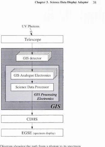
The purpose of the Grazing Incidence Spectrometer (GIS) is to detect UV lines in the wavelength bands discussed in Section 2.4. Figure 3.2 depicts the path from a photon to its spectrum.

A GIS detector consists of MicroChannel Plate (MCP) stacks, which act as an electron multiplier, and a SPiral ANode (SPAN) which receives the electron cloud and provides outputs from which its position to 11-bit resolution in one dimension can be determined. The principle of operation of the GIS is depicted in Figure 3.3.

(39)

UV Photons

T e le sc o p e

GIS detector

GIS Analogu e Electronics jJ ...

Science Data Processor

GIS Processing

Electronics

C D H S

E G S E (spectrum display)

Figure 3.2 Diagram showing the path from a photon to its spectrum.

factor of two; Csl, which is frequently used, is not suitable for use in an open surface arrangement of the GIS (Breeveld and Thomas, 1992). The MCPs operate at a bias voltage of 3.4 kV, and 10% of the M CP voltage is applied between the M CP and the anode.

(40)

electric field

G IS d e te c to r

p (po sitio n )

U V P h o to n

M C P s

p ream ps G IS

P ro cessin g E lectro n ics

M g p2 P h o to c a th o d e

e- ch arg e clo u d 3 m m S P A N an o d e

th ree 8 -bit signals 8-bit an alo g u e to digital co n v ersio n po sitio n d e co d in g lo o k -u p table

11 bit po sitio n

Figure 3.3 Principle of operation of the GIS.

photocathode generating another event in another channel for an M CP in which case there will be two events, which will be treated as simultaneous and will produce errors in position encoding in many readouts, occurring within nanoseconds of each other (Edgar, 1993). Ion feedback can be overcome in Channel Electron M ultipliers (CEMs) by bending (or curving) the tubes as the heavy ions have much longer trajectories than secondary electrons (Edgar, 1993); two stage chevron configuration with zero degree bias front plate (Colson et a i , 1973) and a curved channel or a ‘C ’ plate (Timothy, 1985) can also be used to prevent ion feedback.

(41)

e‘ charge cloud electrodes laser cuts

Figure 3 .4 A 1-D SPAN anode. The width of the electrode triplets has been expanded for clarity. Only five pitches are shown in the figure. The laser cuts separate the electrodes.

throughput as a conventional Wedge and Strip Anode (WSA) was not sufficient to meet the conflicting requirements (Breeveld et a l, 1992a). The SPAN is divided into identical horizontal pitches, and each pitch contains elements (or a fraction) of three electrodes which are sinusoidal, continuous and cyclic (see Figure 3.4). The elements from all the pitches are wire bonded together to make three complete electrodes, X, Y and Z, whose areas have the form of damped sine waves as depicted in Figure 3.4.

3,2.1 GIS Analogue Electronics

Let X , y and z be the magnitudes of charges collected by the electrodes X, Y and Z, respectively. The normalized magnitudes of charges collected on the X- and Y- electrodes (x / (x + y + z) (Z) & y / (x + y + z) (Z)) are unique at any position along the anode; the X- and Y-electrodes are used for measurement and the Z-electrode for normalizing.

(42)

are processed by shaping amplifiers and peak detectors as depicted in Figure 3.5. Tw o of the three analogue outputs (x & y) are digitized by tw o-step flash ADCs (M P7683). As the sum (Z) of all three signals, x, y and z, drives the reference input o f the ADCs, the outputs of the ADCs are two 8-bit values, each of x / Z and y / Z. The sum is also digitized and used directly for building up a PHD. The 16-bit normalized data are then passed to the Science D ata Processor where they are used as the pointing address to a Look Up Table (LUT) for each of four detectors. The complete instm ment subsystem has four detectors, each with its associated read-out electronics.

C h a rg e S h a p in g S h a p in g T ra c k -P e a k M C P A m p s A m p s A m p s A m p s B uffers

&

S P A N

f >

2 -S tep F la s h A D C s

E v e n t T rig g e r

GIS Detectors Z In R ef In R ef

Sum o f C harge

(A D C R ef.)

16 T o S cien ce

D ata P ro cesso r

1.75 X 1 o 'e v e n ls /se c

► Z (fo r P H D ) L evel E v e n t T im in g C o n tro l D is c rim in a to r D is c r im in a to r L ogic

D ead Tim e: 2. l|xs

GIS Analogue Processor

C o n tro l L in es E v e n t C o u n te rs H ig h V o lta g e U n it

Figure 3.5 GIS Analogue Electronics. Each detector has its own associated read-out electronics.

(43)

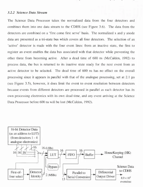
3.2.2 Science Data Stream

The Science D ata Processor takes the normalized data from the four detectors and combines them into one data stream to the CDHS (see Figure 3.6). The data from the detectors are combined on a ‘first come first serve’ basis. The normalized x and y anode data are presented as a tri-state bus which covers all four detectors. The selection of an ‘active’ detector is made with the four event lines: from an inactive state, the first to register an event enables the data bus associated with that detector while preventing the other three from becoming active. After a dead time of 600 ns (McCalden, 1992) to process data, the bus is returned to its inactive state ready for the next event from an active detector to be selected. The dead time of 600 ns has no effect on the overall processing since it appears in parallel with that of the analogue processing, set at 2.1 ps (see Figure 3.5), however, it does limit the event to event resolution between detectors because events from different detectors are processed in parallel as each detector has its own processing electronics with its own dead time, and any event arriving at the Science Data Processor before 600 ns will be lost (M cCalden, 1992).

/ 1 6 16(LSBs)

HouseKeeping (HK) Channel

Science Data to CDHS

2 (MSBs) /►

Bypass

LUT FIFO Buffer

Detector Identity First-of-

four select

Differential Output Driver Parallel to

Serial Conversion 16-bit Detector Data

(as an address to LUT) (from detectors 1 - 4 analogue electronics)

events/sec

(44)

3.2.2.1 Look Up Table

The purpose of the LUT is to take the normalized x and y inputs from the SPAN anode (or GIS Analogue Electronics) and to output the corresponding linear position at which an incoming UV photon hit on the MCP stack (see Figure 3.3). This linear position corresponds to the energy of the incoming photon and hence corresponds to the spectral line energy.

The data from the selected detector must be converted from two-dimensional to linear coordinates with specific calibration characteristics: this is achieved by using a re-loadable LUT for each detector as on-board calculation of the position in one-dimension in real time using a SPAN algorithm (Edgar, 1993) is not possible. This enables the high count rate of over 10^ counts/sec to be processed while minimizing both power and mass; the LUT is pre-calculated based on data from a flat field (Breeveld et a l, 1992a).

In normal use, among the 18 bits of the LUT address, the lower 16-bits of the LUT address are formed from the detector data and the upper two bits from the detector identity (see Figure 3.6) (McCalden, 1992). The LUT outputs 16-bit data among which the Most Significant Bit (MSB), bit 15, is used to inhibit the system output when the information from the detector does not represent a valid position on the anode; bits 13 and 14 are not used at all. The lower 11 bits of the rest (13-bit element) stored in the LUT give a one dimensional event position along the particular detector (a resolution of one part in 2048 pixels), and the other two bits identify that detector. Figure 3.7 depicts the data format. The LUT can be by-passed for detector calibration purposes to allow the raw data (x / E & y / X) to be telemetered (McCalden, 1992).

3.2.2.2 First In First Out Bujfer

(45)

15 14 13 12 11 10

V 9 8 7 6 5 4 3 2 1 0

not used detector

system identification

inhibit

00 : detector 0 01 : detector 1 10 : detector 2 11 : detector 3

positional data

Figure 3.7 Data format from the GIS.

3 .2 .2 3 Other Conversions

A parallel-to-serial conversion is performed on the data from the FIFO, which are fed into the differential output driver to convert the serial data to two differential data streams (inverting and non-inverting) to reject noise. The data are sent to the CDHS at a maximum rate of 8.9 x 10"^ events per second.

3.23 GIS Simulator

The GIS Simulator (GIS_SIM) was designed by McCalden (1991) in the early stage of the project to simulate the whole GIS system, the detector head and the processing electronics, in order to assist the development of the CDHS with the absence of the GIS system. The GIS_SIM was also useful in the development of the SDDA. As it produces three spectral lines per detector at known positions of 0, 1023 and 2047, the performance of the SDDA could be evaluated.

(46)

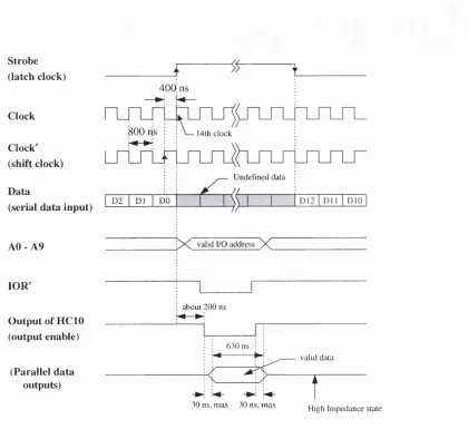
3.3 SDDA SPECIFICATIONS AND REQUIREMENTS

This section describes the SDDA interface with the GIS and its performance specifications and requirements which were set as the result of discussion at a GIS technical meeting at Mullard Space Science Laboratory (MSSL) to provide effective and comprehensive performance evaluation of the GIS detectors.

3.3.1 Interface with the GIS

The data stream from the GIS consists of 13-bit differential serial words each representing a photon position on one of the four detectors, and the two MSBs represent the detector ID number (see Figure 3.7).

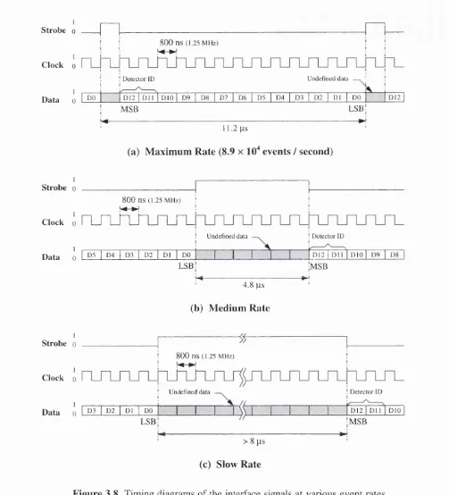
There are two other differential signals that are produced by the GIS, namely, the clock and the strobe. The clock runs at 1.25 MHz which determines the maximum data rate at 8.9 X lO'^ events per second {1 / [(1 / 1.25 MHz) x 14 bit period]}; an event at the

maximum rate takes 14 clock cycles, one clock period to separate two events (see Figure 3.8 (a)). For slower event rates, the period between two events gets longer as depicted in Figure 3.8 (b) and (c). The strobe determines when data are valid; as shown in Figure 3.8, the strobe remains low when data are valid and high when there are null data (dotted portion). Since the data rate varies randomly from 0 to 8.9 x 10"^ events per second, the period between two successive events is also undetermined, i.e., the length of time of the strobe remaining high can be as short as only 800 ns (1 / 1.25 MHz) or as long as several seconds or minutes depending on the valid data rate (see Figure 3.8). A high-to-low transition on the strobe determines the beginning of the data packet (13-bit long GIS data), and a low-to-high transition determines the end of it, as shown in Figure 3.8.

3.3.2 SDDA Performance Requirements

(47)

Strobe o

Clock 0

Data 0

80 0 ns (1.25 M H z) 1

1

1 D etector ID

U ndefined data — . !

1 DO D 12 1 D l l 1 D IO 1 D9 1 D8 D7 1 D6 1 D5 1 D 4 1 D3 I D 2 I D1 1 DO D 12 1

1

^

---M SB L S B |

---►!

11.2 ps

(a) M axim um R ate (8.9 x 10“* events / second)

Strobe o

Clock

80 0 ns (1.25 M H z)

: ruxrLrurun_

Data 0 I D5 I D4 I D 3 I D 2 I D1 I DO I . . . [ . . . ]

LSB

D etector ID U ndefined data

D 12 I D l l I D IO I D 9 I D8

■ 4 .8 p s

(b) M edium Rate

I

Strobe o

Clock 0

8 0 0 ns (1.25 M Hz) I U ndefined data

Data 0 I D3 I D 2 I D1 I DO I j I j

LSB

1 D etector ID

D 12 D l l D IO

M SB > 8 p s

(c) Slow Rate

(48)

The essential SDDA display requirements were as follows:

• To display spectral lines on a PC screen for one detector at a time, with sufficient resolution to display the full 2048 possible line elements (the vertical scale representing the count rates). As a typical PC screen is only 640 pixels wide, the display needs to be wrapped down the screen to make it fit. The 2048 horizontal resolution represents the positions of the dispersed incoming photons along the detectors (i.e. wavelengths of the photons).

• Reduce the resolution of the display to show the spectrum of photons from all four detectors on one screen, ensuring that all lines present are actually displayed. After viewing the whole spectra at the same time, an operator can select one specific detector for the full resolution; the displays can be switched back and forth.

• The vertical scale of the display needs to be switched between logarithmic and linear scales, which range from 0 to 9 x 10"^ events per second. The logarithmic scale provides a better view of the spectrum when the difference in the count rates on different positions along the detector is large, whereas the linear scale is normally used for a precise comparison among different wavelengths or positions along the detectors.

• The maximum on the scale should be operator adjustable to cope with very high or low count rates. The length of the lines (count rates) can be scaled up or down for low or high count rates, respectively, to fit the spectrum within the PC screen window.

• There should be a cursor that, when positioned on a line, displays the line number and the count rate of the line. This feature allows an operator to find out the exact count rates of photons on specific wavelengths.

• The display needs to be printed out. This makes documentation of the results easier. The display can be printed out on HP LaserJet printers.

(49)

exact display with the same options, that are previously saved, is restored, and an operator can apply new options to the display including printing out the display.

• There should be an accumulation mode. In a normal mode, the display is refreshed every half a second (0.52428 seconds, refer to Section 3.4.4.4). In case of low rate data, it is hard to see the spectrum lines even when the lines are scaled up. By accumulating the data without refreshing the screen, low rate data can also be viewed clearly.

• There should be a reference line next to the display. The reference line is set at 3000 counts per second. By comparing the length of the reference hne with the data spectrum lines displayed, it is possible to get a rough idea of the count rates on various positions (1 to 2048) along the detectors without actually halting the process to find out the count rates by placing a cursor on various positions.

• The dead time needs to be calculated and displayed. It is not possible to collect any data from the GIS while the PC is displaying collected data on a screen. The dead time

(%) is given by

Dead Time ( % ) = X 100 % n n

ttotal

where ttotai is the total time taken to collect and process the data and display on a screen and tdispiay is the time taken to process and to display the data. As the data are always collected for 0.52428 seconds (see Sections 3.4 and 3.5 for detail), tdispiay is ttotai - 0.52428 seconds. Therefore, the faster the PC can display data, the shorter the dead time.

3.4 SDDA HARDWARE DESCRIPTION

(50)

As depicted in the block diagram in Figure 3.9, it mainly consists of six blocks: the differential amplifiers to combine two differential (inverting and non-inverting) signal streams into one, the address decoder to select necessary components of the hardware, the serial to parallel converter to enable a simple parallel interface with a PC, the timer (& the external clock) to measure the overall and display time to calculate the dead time, the control logic to inform the PC when and what data to read in, and the PC to display data acquired.

In this section, the function and the use of each block in Figure 3.9 are described in detail.

SD D A

i l l .1 I

A d d ress A 0 -A 9

13.

D a ta

Address Decoder Serial-to-parallel converter D ata

^--- D ata C lock _Differential

^ ---C lock