Vol. 3, Issue 10 (October. 2013), ||V2|| PP 38-47
Effect of Measuring Profile and Metallic Structure on Soil
Resistivity
Mosleh Maeid Al-Harthi
Taif University, KSA
Abstract: - Soil resistivity measurements are considered very important task for grounding system design and analysis. The metallic structures in vicinity of grounding system have significantly effect on the performance of grounding system. Ideally, soil resistivity measurements should be made in the absence of buried metallic conductors or structures. Soil resistivity measurements may have to be made in the presence of the grounding system, if the performance of an existing grounding system is necessary to review or evaluate. Soil resistivity measurements made with the Wenner are carried out with and without a nearby grounding grid, in Taif (KSA) soil. Comparisons are made between the results, with and without the grounding grid, to show the effect due to the presence of the grid. The influence of different metallic structures and modified measurement profiles which reduce the influence of metallic structures will be discussed. A mathematical model for computing the soil resistivity in case of multilayer soil will be investigated. A new technique is proposed to calculate the grounding resistance of multilayer soil by a numerical method as current simulation method.
Index Terms: - Grounding grids, Earth surface potential, Step voltage, Touch voltage, Boundary element method, Charge simulation method, current simulation method.
I.
INTRODUCTION
The objectives of adequate grounding system are summarized in the following points: Creating an easy return path for the return stroke current that develops from lightning, Reduction the breakdown risks on electrical and electronic equipments, Achievement the minimum cost by continuity of the power systems and Reduction the risks for human by decreasing the touch and step voltages which are the most parameters for grounding system.
The resistance of a driven earth electrode is determined by the resistivity of the soil, which is influenced by various factors including moisture content, soil temperature and the depth of the electrode. Soil resistivity measurements taken at the intended site provide a valuable insight into how the desired earth resistance value can be achieved and maintained over the life of the installation, with the minimum cost and effort. The purpose of resistivity testing is to obtain a set of measurements that can be interpreted to yield an equivalent model for the electrical performance of the earth, as seen by the particular earthing system. However, the results may be incorrect or misleading if adequate investigation is not made prior to the test or the test is not correctly undertaken.
Earth resistivity measurement interpretation techniques as part of a major EPRI research project on transmission line grounding are developed [1]. The interpretation techniques include graphical curve matching and an advanced computer program (RESIST). The curve matching technique requires a set of theoretical Master Curves with which a field curve can be compared directly. Program RESIST is based on the analytical methods used in a more elaborate computer program which has been in operation for several years. For an electrode spacing of 2.5 meters or greater, satisfactory agreement is obtained between measured and computed results using both interpretation techniques.
An expression of apparent resistivity for multilayer earth structure is developed in [2]. This expression helps in editing the -a curve for an arbitrary number of layers. They compared the -a curve from their
-a curve and the results showed good agreement for two case studies.
A novel calculation method for the parameters of the two-layer soil model is presented in [3]. The proposed method is valid for an arbitrary number of soil layers with arbitrary values of resistivity, and it is applicable to simple as well as complex grounding systems. The numerical results of this method were compared with electromagnetic field calculations carried out with a computer program based on the finite-element method. The proposed model permits the use of computer programs based on the method of images and a two-layer soil model for the design of station grounding systems buried in horizontal multilayer soil stratifications.
formulae for uniform soil to account for the multi-layer soil structure. A comparative analysis of available expressions for uniform and two-layer soils is performed in order to check their applicability in various cases. A method for the estimation of soil parameters in the case of a multilayered horizontal soil is investigated in [5]. The method is used in education for the interpretation of resistivity sounding measurements of a stratified soil. A graphical interface is utilized and allows the users to interact during geophysical inversion and provides feedback in the form of apparent resistivity curves along with information on the progression of the process. The use of an interactive tool for the interpretation of resistivity sounding was demonstrated in [5]. Interpretation of measurements is done by minimizing the quadratic, relative or logarithmic distance between the measured and the calculated resistivities. They concluded that a graphical interface has proven to be an efficient tool for introducing concepts in resistivity sounding.
Soil resistivity parameters of two-layer vertical soil as a one of the practical soil models are studied and estimated in [6]. Wenner method is used to measure the apparent soil resistivity. To achieve this study, the image method is proposed to consider the presence of vertical layer soil and four electrodes of the Wenner method. A general apparent resistivity expression is proposed to find the relation between the apparent resistivity and the four electrodes of Winner method locations and soil parameters. The proposed equation with the aid of Gauss-Newton method is used to estimate the soil parameters.
The influence of buried metallic structures on soil resistivity measurements is studied [7]. They analyzed different measurement methods, various soil structures, and different locations of measurement profiles with respect to metallic structures. This study also shows how to choose measurement locations to minimize the influence of buried metallic structures when soil resistivity measurements must be made in the presence of buried metallic structures.
This paper will present a new application of the current simulation method to calculate the grounding resistance of multilayer soil. The real test to measure the soil resistivity is made using Wenner method to study the effect of metallic structures on the resistivity value. Also the effect of the measuring profile on the resistivity value is investigated.
II.
PROBLEM IDENTIFICATION
The problem for calculating the grounding resistance of multi-soil is how the apparent resistivity can be calculated. As in [8], the apparent resistivity for two soil model calculates by the following formula;
1 2 2 1 2 1
1
for
1
1
1
0
h d K ae
(1) 1 2 2 1 1 22
1
1
1
0for
h d K ae
(2) Where, d0 is the depth to the boundary of the zones, K is the reflection factor (K=( ρ2- ρ1)/ ( ρ1+ ρ2)) and h isthe top layer depth.
Equations (1) and (2), are valid for the boundary depth greater than or equal the grid depth. But in [4], Eq. (2) is modified because at very large depth of upper soil layer, resistivity a given by Eq. (2) tends to 2.
This is physically incorrect if the electrode lies in the upper soil layer, as assumed in [8]. Therefore, Eq. (2) is modified [4] as follows:
1 2 2 1 1 2
1
1
1
1
0for
h d K ae
(3) For finite h and very large d0, resistivity a given by Eq. (3) tends to 1, which is in compliance with physicalreasoning.
III.
CURRENT SIMULATION METHOD IN TWO-LAYER SOIL
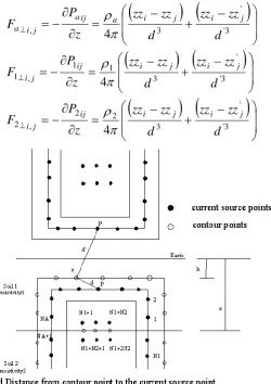
As in the Current Simulation Method, the actual electric filed is simulated with a field formed by a number of discrete current sources which are placed outside the region where the field solution is desired. Values of the discrete current sources are determined by satisfying the boundary conditions at a selected number of contour points. Once the values and positions of simulation current sources are known, the potential and field distribution anywhere in the region can be computed easily [10].
The field computation for the two-layer soil system is somewhat complicated due to the fact that the dipoles are realigned in different soils under the influence of the applied voltage. Such realignment of dipoles produces a net surface current on the dielectric interface. Thus in addition to the electrodes, each dielectric interface needs to be simulated by fictitious current sources. Here, it is important to note that the interface boundary does not correspond to an equi-potential surface. Moreover, it must be possible to calculate the electric field on both sides of the interface boundary.
In the simple example shown in Figure 1, there are N1 numbers of current sources and contour points to simulate the electrode, of which NA are on the side of soil A and (N1- NA) are on the side of soil B. These N1
current sources are valid for field calculation in both soils. At the different soil interface there are N2 contour
points (N1 +1,….., N1+N2), with N2 current sources (N1+1,…..,N1+N2) in soil A valid for soil B and N2
current sources (N1+N2+1,…..,N1+2N2) in soil B valid for soil A. Altogether there are (N1+N2) number of
contour points and (N1 + 2N2) number of current sources.
As in Figure 1, h is the grid depth and z is the depth of top layer soil. In order to determine the fictitious current sources, a system of equations is formulated by imposing the following boundary conditions.
At each contour point on the electrode surface the potential must be equal to the known electrode potential. This condition is also known as Dirichlet’s condition on the electrode surface.
At each contour point on the dielectric interface, the potential and the normal component of flux density must be same when computed from either side of the boundary.
Thus the application of the first boundary condition to contour points 1 to N1 yields the following equations.
1 1 , 2 1 , 2
1 1, 1 ,
,
1
...
,
1
...
2 1 ! 1 2 1 2 ! 1N
N
i
V
I
P
I
P
N
i
V
I
P
I
P
A N N N j j j i N j j j i a A N N N Nj i j j
N
j ai j j
(4) where,
' 2 , 2 ' 1 , 1 ' ,1
1
4
1
1
4
,
1
1
4
d
d
P
d
d
P
d
d
P
j i j i a j i a
Again the application of the second boundary condition for potential and normal current density to contour points = N1+1 to N1+N2 on the dielectric interface results into the following equations. From potential continuity
condition: 2 1 1 2
1 1, 1 2 ,
,
1
....
0
2 1 2 ! 2 1 1N
N
N
i
I
P
I
P
N N N Nj i j j
N N
N
j i j j
(5) From continuity condition of normal current density Jn:
J
n1
i
J
n2
i
0
for
i
N
1
1
,
N
1
N
2 (6) Eqn. (6) can be expanded as follows:
3 ' ' 3 2 2 , 2 3 ' ' 3 1 1 , 1 3 ' ' 3 ,4
4
4
d
zz
zz
d
zz
zz
z
P
F
d
zz
zz
d
zz
zz
z
P
F
d
zz
zz
d
zz
zz
z
P
F
j i j i ij j i j i j i ij j i j i j i a ij a j i a
Fig. 1: Fictitious current source with contour points for field calculation by current simulation method in two-layer soil
where, F┴,ij is the field coefficient in the normal direction to the soil boundary at the respective contour point, ρa, ρ1 & ρ2 are the apparent resistivity nd resistivities of soil 1 and 2 respectively and zzi & zzj are
the dimension of the contour point and current source in z direction respectively. Equations 4 to 7 are solved to determine the unknown fictitious current sources.
After solving 4 to 7 to determine the unknown fictitious current source points, the potential on the earth surface can be calculated by using Eq. 4. Also, the ground resistance (Rg) can be calculated using the following
equation:
1 1 N j gI
V
R
(8) where, V is the voltage applied on the grid which is assumed 1V.When the boundary depth is lower than the grid depth, the apparent resistivity tends to 2. Therefore,
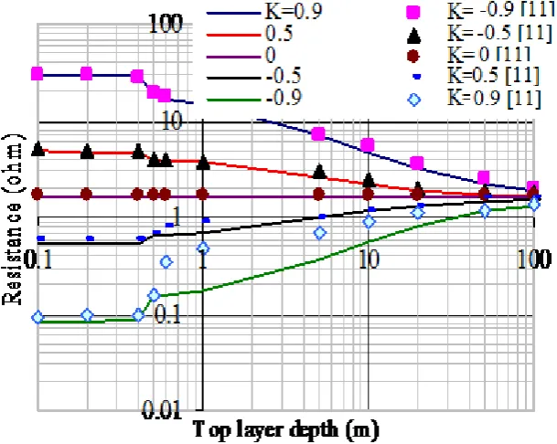
by using Eq. 1 and 3 for calculating the grounding resistance by Current Simulation Method, the large different between the proposed method results and the results in [11] is observed for K<-0.5 and this shown in Figure 2. If Eq. 3 is modified as in 9 the results by the proposed method are good agreement with the results in [11].
1 2 15 1 1 2
1
1
1
1
for
0
Fig. 2: Relation between 4 meshes grid resistance and the top layer depth
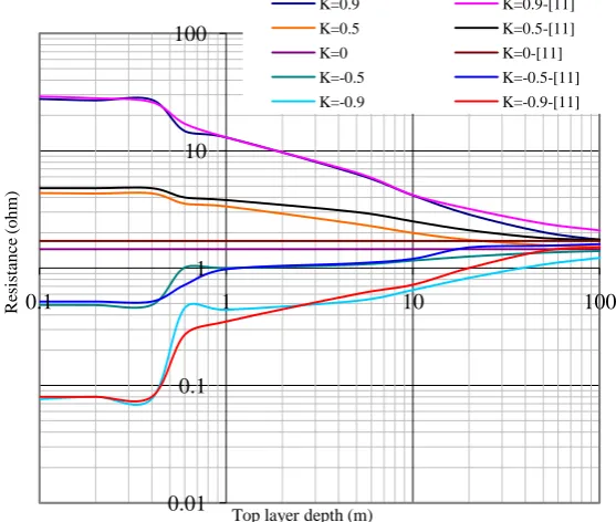
Figures 3 and 4 present the comparison of the results calculated by the proposed method with the results reported in [11] for a square 30m*30m, 4 and 16 meshes grids buried at 0.5 m depth in various two layer structures. It is noticed from Figs. 3 and 4 that the proposed method gives a good agreement with the results in [11].
0.01 0.1 1 10
0.1 1 10 100
R
e
si
st
a
n
c
e
(
o
h
m
)
Top layer depth (m)
K=0.9 K=0.9-[11] K=0.5 K=0.5-[11]
K=0 K=0-[11]
K=-0.5 K=-0.5-[11] K=-0.9 K=-0.9-[11]
0.01 0.1 1 10 100
0.1 1 10 100
R
esi
st
an
ce
(
o
h
m)
Top layer depth (m)
K=0.9 K=0.9-[11]
K=0.5 K=0.5-[11]
K=0 K=0-[11]
K=-0.5 K=-0.5-[11]
K=-0.9 K=-0.9-[11]
Fig. 4: Relation between 16 meshes grid resistance and the top layer depth
IV.
EFFECT OF THE METALLIC STRUCTURE ON THE GROUNDING RESISTIVITY
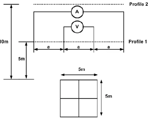
The Wenner array as shown in Figure 5 is the least efficient from an operational perspective. It requires the longest cable layout, largest electrode spreads and for large spacings one person per electrode is necessary to complete the survey in a reasonable time. Also, because all four electrodes are moved after each reading the Wenner Array is most susceptible to lateral variation effects.
However, the Wenner array is the most efficient in terms of the ratio of received voltage per unit of transmitted current. Where unfavourable conditions such as very dry or frozen soil exist, considerable time may be spent trying to improve the contact resistance between the electrode and the soil.
Fig. 5: Wenner four pin soil resistivity test set-up
The Wenner four-pin method, as shown in figure above, is the most commonly used technique for soil resistivity measurements. Using the Wenner method, the apparent soil resistivity value is:
2
4
2 2 22
1
4
b
a
a
b
a
a
aR
W E
(10) Where, E=measured apparent soil resistivity (m), a=electrode spacing (m), b=depth of the electrode
penetrating the ground only for a short distance (as normally happens), the previous equation can be reduced to
E
2
aR
W.A. On Site Work
In the first, the land is chosen beside the university and the metallic structures are made and brought to the site to start the test. Figures 6 and 7 show the test setup and the measuring profiles and its distance from the metallic structure (two configurations grid, the first is 16 meshes grid and the other is 4 meshes grid)
Fig. 6: 16 meshes grid and the measuremet profiles
After putting the grids in the soil, the measurements have been carried out using Earth resistance and earth resistivity test device KEW 4106 to study the effect of the metallic structure on the soil resistivity as shown in the following pictures;
After preparing the setup of the test, the reading will be collocted as shown in the next pictures;
V.
MEASUREMENT RESULTS
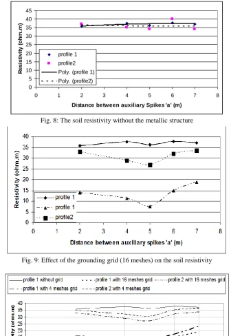
Fig. 8: The soil resistivity without the metallic structure
Fig. 9: Effect of the grounding grid (16 meshes) on the soil resistivity
Fig. 10: Effect of the grounding grid configurations on the soil resistivity
VI.
CONCLUSIONS
This project aims to calculate the grounding resistance of multilayer soil by the Current Simulation Method. The validation of the method is satisfying by a comparison between the results from the method and the results in [18]. It is seen that a good agreement between the proposed method results and the results in [18]. Also study the effect of the metallic structure on the resistivity of the soil.
Without the grid, the average “measured” soil resistivities for all spacings are 35000 ohm.m.
With the grid, the “measured” resistivities, shown, are generally lower.
The resistivity curve corresponding to the case without the grid is a horizontal line as expected.
0 5 10 15 20 25 30 35 40 45
0 1 2 3 4 5 6 7 8
Distance between auxiliary Spikes 'a' (m)
R
e
s
is
ti
v
it
y
(
oh
m
.m
)
profile 1
profile2
Poly. (profile 1)
The resistivity curves corresponding to cases with the grid present are no longer straight lines and the degree of deviation from the horizontal line shows the degree of influence of the grounding grid.
for Profile 1, which is close to the grid, the deviation is the largest. When the profile is moved away from the grid, as in the case of Profile 2, the deviation is much smaller.
It is noted that for measurements along Profile 1, the largest deviation occurs when the current probe spacing is equal to the length of the grid (5m).
REFERENCES
[1] F. Dawalibi, C. J. Blattner “Earth resistivity measurement interpretation techniques”, IEEE Transactions on Power Apparatus and Systems, Vol. PAS-103, No. 2, February 1984, pp. 374-382.
[2] T. Takahashi, T. Kawase "Analysis of apparent resistivity in a multi-layer earth structure" IEEE Transaction on Electrical Insulation, Vol. 5, No. 2, April 1990, pp 604-612.
[3] Enrique Mombello, Oscar Trad, Jorge Rivera, Albert0 Andreoni," Two-layer soil model for power station grounding system calculation considering multilayer soil stratification", Electric Power Systems Research 37 (1996), pp. 67-78.
[4] Jovan Nahman , Ivica Paunovic, "Resistance to earth of earthing grids buried in multi-layer soil", Electrical Engineering (2006) 88: pp. 281–287.
[5] Lagace, P.J. , Vuong, M.H. "Graphical User Interface for Interpreting and Validating Soil Resistivity Measurements" IEEE ISIE 2006, July 9-12, 2006, Montreal, Quebec, Canada, pp. 1841-1845.
[6] Nayel,Mohamed Lu,Boyang ; Tian,Yu ; Zhao,Yingzhen, "Study of Soil Resistivity Measurements in Vertical Two-Layer Soil Model", IEEE APPEEC 2012, March 27-29, 2012, pp. 1-5.
[7] J. Ma, Member, IEEE F. P. Dawalibi, " Study of influence of buried metallic structures on soil resistivity measurements“, IEEE Transactions on Power Delivery, Vol. 13, No. 2, April 1998, pp. 356-365.
[8] J. A. Sullivan "Alternative earthing calculations for grids and rods" IEE Proc. Gener. Transm. Distvib, Vol.145, No.3, May 1998.
[9] Cheng-Nan Chang, Chien-Hsing Lee, “ Compuation of ground resistances and assessment of ground grid safety at 161/23.9 kV indoor/tzpe substation”, IEEE Transactions on Power Delivery, Vol. 21, No. 3, pp. 1250/1260, July 2006.
[10] N. H. Malik, “A review of charge simulation method and its application,” IEEE Transaction on Electrical Insulation, vol. 24, No. 1, February 1989, pp 3-20.