Higher order binaries with time dependent coefficients and two factors

(1)

-model for defaultable bond with discrete default information

Hyong-Chol O

a,∗

,

Yong-Gon Kim

a

and Dong-Hyok Kim

a

a_{Faculty of Mathematics,}_{Kim Il Sung}_{University, Pyongyang, D.P.R Korea}

Abstract

In this article, we consider a 2 factors-model for pricing defaultable bonds with discrete default intensity and barrier where the 2 factors are a stochastic risk free short rate process and firm value process. We assume that the default event occurs in an expected manner when the firm value reaches a given default barrier at predetermined discrete announcing dates or in an unexpected manner at the first jump time of a Poisson process with given default intensity given by a step function of time variable. Then our pricing model is given by a solving problem of several linear PDEs with variable coefficients and terminal value of binary type in every subinterval between the two adjacent announcing dates. Our main approach is to use higher order binaries. We first provide the pricing formulae of higher order binaries with time dependent coefficients and consider their integrals on the last expiry date variable. Then using the pricing formulae of higher binary options and their integrals, we give the pricing formulae of defaultable bonds in both cases of exogenous and endogenous default recoveries and perform credit spread analysis.

Keywords: higher order binary options, time dependent coefficients, defaultable bond, default intensity, default barrier, exogenous, endogenous, credit spread.

1

Introduction

The study on defaultable corporate bonds and credit risk is now one of the most promising areas of cutting edge in financial mathematics [1]. As well known, there are two main approaches to pricing defaultable corporate bonds; one is the structural approach and the other one is the reduced form approach. In the structural method, we think that the default event occurs when the firm value is not enough to repay debt, that is, the firm value reaches a certain lower threshold (default barrier) from above. Such a default can be expected and thus we call it expected default. In the reduced-form approach, the default is treated as an unpredictable event governed by a default intensity process. In this case, the default event can occur without any correlation with the firm value and such a default is calledunexpected default. In the reduced-form approach, if the default probability in time interval[t,t+∆t]isλ∆t, thenλis calleddefault intensityorhazard rate.

As for the history of the two approaches and their advantages and shortcomings, readers can refer to the introductions of [5, 8, 9, 13, 19]. To take the advantages and overcome the shortcomings of structural and reduced-form approaches, many authors used unified models of the two approaches. (See [5, 6, 8, 9, 13, 14, 17, 18, 19, 20].) As noted in [14, 17, 18], many researchers of unified model including [5, 6, 8, 9, 13, 19] tried to express the price of the bond in terms of the firm value or the related signal variable to the firm value and the value of default intensity together with default barrier at any time in the whole lifetime of the bond.

On the other hand, Duffie et al. [10] observe that it is typically difficult for investors in the secondary market for corporate bonds to observe a firm’s assets directly, because of noisy or delayed accounting reports,

∗_{Corresponding author.}

(2)

or barriers to monitoring by other means. In [14, 17] the authors noted that it is difficult for investors outside the firm to know the firm’s financial data except for some discrete dates (for example, once in a month or once in a three month etc.) to announce management data and studied the pricing problem for defaultable corporate bond under the assumption that we only know the firm value and the default barrier at 2 fixed discrete announcing dates, we don’t know about any information of the firm value in another time and the default intensity between the adjoined two announcing dates is a constant determined by its announced firm value at the former announcing date. The computational error in [17] is corrected in [14]. The approach of [14, 17] is a kind of study of defaultable bond under insufficient information about the firm. It is interesting to note that E. Agliardi et al. [2, 3] studied bond pricing problem under imprecise information with the technique of fuzzy mathematics. The approach of [14, 17] can also be seen as a unified model of structural model and reduced form model. Agliardi [1] studied a structural model for defaultable bond with several (discrete) coupon dates where the default can occur only when the firm value is not large enough to pay its debt and coupon in those discrete coupon dates.

In [18], the authors studied a one-factor model for defaultable bond with discrete default intensity and discrete default barrier using higher order binary options and their integrals, where the 1 factor is the firm value process. In their credit risk model, the default event occurs in an expected manner when the firm value reaches a certain lower threshold - the default barrier at predetermined discrete announcing dates or in an unexpected manner at the first jump time of a Poisson process with given default intensity given by a step function of time variable, respectively. They considered both endogenous and exogenous default recovery and the pricing model is a solving problem of inhomogeneous or homogeneous Black-Scholes PDEs with different coefficients and terminal value of binary type in every subinterval between the two adjacent announcing dates. In order to deal with the inhomogenous term related to endogenous recovery, they introduced a special binary option called integral of i-th binary or nothing and using it obtained the pricing formulae of defaultable corporate bond. The approach of [18] to model credit risk seems similar with the one of [14] but the essential difference is that in [14] they assumed that they know the firm value only in the discrete announcing dates and the default intensity between two adjacent announcing dates is determined by the firm value in the former announcing date. Another different point is that [18] considered arbitrary number of announcing dates while [14] considered only 2 announcing dates.

As a continued study of [18] we here consider a two factors - model for pricing defaultable bond with discrete default intensity and barrier where the 2 factors are stochastic risk free short rate process and firm value process. Our pricing model is given by a solving problem of several PDEs with variable coefficients and terminal value of binary type in every subinterval between the two adjacent announcing dates. Through the change of numeraire, they are transformed into several homogeneous or inhomogeneous Black-Scholes PDEs with different time dependent coefficients and terminal value of binary type. The coefficients time dependency is the different point from [18]. Here we encounter the problems of higher order binaries with time dependent coefficients even if the drifts and volatilities of short rate and firm value processes are all constants. Therefore we first provide the pricing formulae of higher order binaries with time dependent coefficients and consider their integrals on the last expiry date variable. Then using the pricing formulae of higher binary options and their integrals, we give the pricing formulae of defaultable bonds in both cases of exogenous and endogenous default recoveries and credit spread analysis.

Finally we note that it is interesting to see that the Geske’s compound option approach used in [1] for pricing of defaultable bond with discrete coupon payments in structural approach is the same technique as higher binary used here.

The remainder of the article is organized as follows. In section 2 we consider higher order binaries with time dependent coefficients and their properties. In section 3 we set the problem for defaultable bonds and provide the pricing formulae and credit spread analysis. In section 4 we provide the sketch of the proof of pricing formulae for defaultable bonds.

2

Higher order binaries with time dependent coefficients

(3)

volatilityσ(t).

∂V ∂t

+σ 2₍_t₎

2 x

2∂2V

∂x2

+ (r(t)−q(t))x∂V

∂x

−r(t)V=0, 0≤t<T, 0<x<∞, (2.1)

V(x,T) =x·1(sx>sξ), (2.2)

V(x,T) =1(sx>sξ). (2.3)

Heres=±1 and the signs refer to the call/put attribute of the option.

The solution to the problem (2.1) and (2.3) is called theasset-or-nothing binaries(orassetbinaries) and de-noted byAs_ξ(x,t;T). The solution to the problem (2.1) and (2.3) is called thecash-or-nothing binaries(orbond bi-naries) and denoted byBs_ξ(x,t;T). Asset binary and bond binary are called thefirst order binaryoptions. If nec-essary, we will denote byAs_ξ(x,t;T;r(·),q(·),σ(·))orBs_ξ(x,t;T;r(·),q(·),σ(·)), where the coefficientsr(t),q(t) andσ(t)of Black-Scholes equation (2.1) are explicitly included in the notation.

Let assume that 0 < T0 < T1 < · · · < Tn−1 and the (n−1)th order (asset or bond) binary options

As1···sn−1

ξ1···ξn−1(x,t;T1,· · ·,Tn−1)andB

s1···sn−1

ξ1···ξn−1(x,t;T1,· · · ,Tn−1)are already defined. Let

V(x,T0) =A_ξs1₁···s···ξnn−−11(x,T0;T1,· · ·,Tn−1)·1(s0x>s0ξ0), (2.4)

V(x,T0) =B_ξs1₁···s_···_ξn_n−₋1₁(x,T0;T1,· · · ,Tn−1)·1(s0x>s0ξ0), (2.5)

The solution to the problem (2.1) and (2.4) is called then-th order asset binariesand denoted byAs0s1···sn−1

ξ0ξ1···ξn−1(x,t;T0,

T1,· · ·,Tn−1). The solution to the problem (2.1) and (2.5) is called then-th order bond binariesand denoted by

Bs0s1···sn−1

ξ0ξ1···ξn−1(x,t;T0,T1,· · · ,Tn−1).

Next, we provide the pricing formulae of asset and bond binaries with time dependent coefficients. In the sequel the terminal value of the option price is a given function f(x), that is

V(x,T) = f(x). (2.6)

Lemma 2.1. Assume that there exist nonnegative constants M andαsuch that|f(x)| ≤ Mxαlnx,x >0. Then the

solution of(2.1)and(2.6)is provided as follows:

V(x,t;T) =e−r(t,T)

Z ∞

0

1 q

2πσ2₍_t_,_T₎

1

ze

−(ln x

z+r(t,T)−q(t,T)−12σ2(t,T)) 2

2σ2(t,T) _f₍_z₎_dz

=xe−q(t,T)

Z ∞

0

1 q

2πσ2₍_t_,_T₎

1

z2e −(ln

x

z+r(t,T)−q(t,T)+12σ2(t,T)) 2

2σ2(t,T) _f₍_z₎_dz_. _(2.7)

Here

r(t,T) =

Z T

t

r(s)ds, q(t,T) =

Z T

t

q(s)ds, σ2(t,T) = Z T

t

σ2(s)ds. (2.8)

Proof. It is well known that the solution to Black-Scholes equation with time dependent coefficientsr(t),q(t)

andσ(t)can be obtained by replacingr(T−t),q(T−t)andσ2(T−t)in the solution representation of Black-Scholes equation with constant coefficientsr,qandσintor(t,T),q(t,T)andσ2(t,T). Using this fact and the proposition 1 at page 249 in [15], we soon have (2.7). A way of direct proof is as follows. As in [12], in (2.1) we use the changes of variable and unknown function . Then (2.1) is changed to

     ∂U

∂t +

1

2σ2(t)y2∂

2_U

∂y2 =0, 0<t<T, y>0,

U(y,T) = f(y), y>0.

If we change time variable intoτ=R₀tσ2(s)ds, ˆT=R₀Tσ2(s)ds, then we have      ∂U ∂τ + 1 2y2∂

2_U

∂y2 =0, 0<τ<Tˆ, y>0,

(4)

This is the Black-Scholes equation with constant coefficients 0, 0 and 1 and thus we apply the proposition 1 at page 249 in [15] to get the representation ofU(y,τ). Returning to original variables and unknown function, we get (2.7).

Theorem 2.1. (The Pricing Formulae of Higher Order Binary Options with Time Dependent Coefficients)The

prices of higher order bond and asset binaries with risk free short rate r(t), dividend rate q(t)and volatilityσ(t)are as

follows.

As_K(x,t;T;r(·),q(·),σ(·)) =xe−q(t,T)N(sd),

Bs_K(x,t;T;r(·),q(·),σ(·)) =e−r(t,T)N(sd0), s= +or−, (2.9)

N(x) =√2π−1 Z x

−∞exp[−y

2_/2_]_dy_,

d=

q

σ2(t,T) −1_h

ln(x/K) +r(t,T)−q(t,T) +σ2(t,T)/2 i

, d0=d−

q

σ2(t,T),

As1s2

K1K2(x,t;T1,T2) =xe

−q(t,T2)_N₂₍_s₁_d₁_,_s₂_d₂_;_s₁_s₂_ρ₎_,

Bs1s2

K1K2(x,t;T1,T2) =e

−r(t,T2)_N₂₍_s₁_d0

1,s2d02;s1s2ρ), s1,s2= +or−,

(2.10)

N2(a,b;ρ) = Z a −∞ Z b −∞ 2π q 1−ρ2

−1

e−

y2−2ρyz+z2

2(1−ρ2) _dydz_,

ρ= q

σ2(t,T1)/σ2(t,T2),

As1···sm

ξ1···ξm(x,t;T1,· · · ,Tm) =xe

−q(t,Tm)_N_m₍_s

1d1,· · · ,smdm;As1···sm), si= +or−,m≥3,

Bs1···sm

ξ1···ξm(x,t;T1,· · ·,Tm) =e

−r(t,Tm)_N_m₍_s

1d01,· · ·,smd0m;As1···sm), i=1,· · ·,m,

(2.11)

Nm(a1,· · · ,am;A) =

Z a1

−∞· · · Z am

−∞ 1

√

2πm

√

detAexp

−1

2y

⊥_Ay_dy_,

di=

q

σ2(t,Ti)

−1

h

ln(x/Ki) +r(t,Ti)−q(t,Ti) +σ2(t,Ti)/2

i ,

d0_i=di−

q

σ2(t,Ti), i=1,· · ·,m,

As₁···sm = (sisjaij) m i,j=1.

Here y⊥= (y1,· · ·,ym)and the matrix aijm_i,j₌₁is given as follows:

a11 =σ2(t,T2)/σ2(T1,T2), amm =σ2(t,Tm)/σ2(Tm−1,Tm),

aii=σ2(t,Ti)/σ2(Ti−1,Ti) +σ2(t,Ti)/σ2(Ti,Ti+1), 2≤i≤m−1,

ai,i+1=ai+1,i =−

q

σ2(t,Ti)·σ2(t,Ti+1)/σ2(Ti,Ti+1), 1≤i≤m−1,

aij=0 for anotheri,j=1,· · · ,m.

Proof. As_K(x,t;T)is just the solution to the problems (2.1) and (2.6) whenf(x) =x·1(sx>sK). If we substitute

f(x) =x·1(sx>sK)into the second formula of (2.7), we soon get the formula forAs_K(x,t;T)of (2.9). Similarly, if we substitute f(x) = 1(sx > sK)into the first formula of (2.7), we soon get the formula forBs_K(x,t;T)of (2.9).

As1s2

K₁K2(x,t;T1,T2)is just the solution to the problems (2.1) and (2.6) whenT=T1andf(x) =A

s2

K2(x,T1;T2)·

1(s1x > s1K1). If we substitute f(x) = AsK22(x,T1;T2)·1(s1x > s1K1)and the formula for A

s2

K2(x,T1;T2)of

(2.9) into the second formula of (2.7) and represent the integral with the cumulative distribution function of bivariate normal distribution, we get the formula for As1s2

K1K2(x,t;T1,T2)of (2.10). Similarly, if we substitute

f(x) = Bs2

K2(x,T1;T2)·1(s1x > s1K1)and the formula forB

s2

K2(x,T1;T2)of (2.9) into the first formula of (2.7)

and represent the integral with the cumulative distribution function of bivariate normal distribution, we get the formula forBs1s2

K1K2(x,t;T1,T2)of (2.10).

In the case ofm>2, we use induction to prove (2.11). Assume that (2.11) holds form=n−1. Then from (2.4)As1s2···sn

ξ1ξ2···ξn(x,t;T1;T2,· · · ,Tn)satisfies (2.1) whenT=T1and

(5)

Then from the second formula of (2.7),As1s2···sn

ξ1ξ2···ξn(x,t;T1,T2,· · · ,Tn)is provided as follows:

As1s2···sn

ξ1ξ2···ξn(x,t;T1,T2,· · ·,Tn) =xe−q(t,T1)

Z ∞

0

1 q

2πσ2₍_t_,_T 1)

1

z2e −(ln

x

z+r(t,T1)−q(t,T1)+12σ2(t,T₁))2

2σ2(t,T₁) _As2···sn

ξ2···ξn(z,T1;T2,· · ·,Tn)·1(s1z>s1ξ1)dz.

HereAs2···sn

ξ2···ξn(z,T1;T2,· · ·,Tn)is the price of the underlying(n−1)-th order asset binary option and thus by

induction-assumption and (2.11) we have

As2···sn

ξ2···ξn(z,T1;T2,· · ·,Tn) =ze

−q(T1,Tn)_N

n−1(s2d2,· · ·,sndn;As2···sn).

If we substitute this equality into the above integral representation and represent the integral with the cumu-lative distribution function ofn-variate normal distribution, we can get the first formula of (2.11) form=n. The result for bond binaries (the second formula of (2.11)) is similarly proved.

Remark 2.1. Recently (higher order) binary options were priced in the literature, in particular, in [11] the Black-Scholes framework was adopted and in [4] the more general L´evy framework was studied. Theorem 2.1 is a generalization of the corresponding results of [7, 15]. In Theorem 2.1, N2(a,b;ρ)is the cumulative distribution function of bivariate

nor-mal distribution with a mean vector [0, 0] and a covariance matrix[1,ρ;ρ, 1](symbols in the software “Matlab”), and Nm(a1,· · ·,am;A)is the cumulative distribution function of m-variate normal distribution with zero mean vector and

a covariance matrix A−1= rijm_i,j₌₁where rij=

q

σ2(t,Ti)/σ2(t,Tj), rji=rij, i≤j. Such special functions can

eas-ily be calculated by standard functions supplied in standard software for mathematical calculation (for example, Matlab).

Next, we consider a relation between prices of higher order binaries with constant difference between risk free rates and dividend rates. From the formulae (2.9), (2.10) and (2.11), whenbis a constant, we have:

As1···sm

K₁···Km(x,t;T1,· · ·,Tm;r1(·),r1(·) +b,σ(·)) =e

−(r1−r2)(t,Tm)_As1···sm

K₁···Km(x,t;T1,· · · ,Tm;r2(·),r2(·) +b,σ(·)),

Bs1···sm

K1···Km(x,t;T1,· · ·,Tm;r1(·),r1(·) +b,σ(·)) =e

−(r1−r2)(t,Tm)_Bs1···sm

K1···Km(x,t;T1,· · · ,Tm;r2(·),r2(·) +b,σ(·)).

(2.12)

Next, as in [18], we can prove the following lemma. The proof is easy and omitted.

Lemma 2.2. (Integral of binary or nothing)Assume that g(τ)is a continuous function ofτ∈[Ti−1,T]. Let

V(x,T0) = 1(s0x>s0ξ0)

Z T

Ti−1

g(τ)·F_ξs1···si−1si

1···ξi−1ξi(x,T0;T1,· · ·,Ti−1,τ)dτ. (2.13)

Then the solution of(2.1)and(2.13)is given as follows:

V(x,t) =

Z T

Ti−1

g(τ)·F_ξs0s1···si−1si

0ξ1···ξi−1ξi(x,t;T0,T1,· · ·,Ti−1,τ)dτ. (2.14)

Here F=A or F=B.

3

The problem of defaultable bonds with discrete default information, the pricing

for-mulae and credit spread analysis

3.1 The problem

Assumptions: 1) Short rate follows the law

drt=ar(r,t)dt+sr(t)dW1(t), ar(r,t) =a1(t)−a2(t)r (3.1)

(6)

2) 0 = t0 < t1 < · · · < tN−1 < tN = T, t1,· · · ,tN are announcing dates and T is the maturity of

our corporate bond with face value 1 (unit of currency). For everyi = 0,· · ·,N−1 the unexpected default probability in[t,t+dt]T_[

ti,ti+1]isλidt. Here the default intensityλiis a constant.

3) The firm valueV(t)follows a geometric Brown motiondV(t) = (rt−b)V(t)dt+sV(t)V(t)dW2(t)under

the risk neutral martingale measure and a standard Wiener process W1 and E(dW1,dW2) = ρdt. The firm continuously pays out dividend in rateb(constant) for a unit of firm value.

4) The expected default barrier is only given at timetiand the expected default event occurs when

V(ti)≤KiZ(r,ti;T) (i=1,· · ·,N).

HereKiis a constant that reflects the quantity of debt andZ(r,t;T)is default free zero coupon bond price.

5) The expected default recovery Red is given by Re·Z(r,t;T), the unexpected default recovery Rud as

Ru·Z(r,t;T)and the recovery rates 0≤Re,Ru≤1 are constants. (Exogenousrecovery.)

5)’ The expected default recovery is given byRed =Re·α·V, the unexpected default recovery byRud =

min{Z(r,t), Ru·α·V}and the recovery rates 0 ≤Re,Ru ≤1 are constants and 0<α <1 is a constant that reflects the quantity of debt (Endogenousrecovery). Here the reason why the expected default recovery and unexpected recovery are given in different forms is to avoid the possibility of paying more than the current price of risk free bond as a default recovery when the unexpected default event occurs.

6) In the subinterval(ti,ti+1), the price of our corporate bond is given by a sufficiently smooth function

Ci(V,r,t)(i=0,· · · ,N−1).

Problem. Find the representation of the price functionCi(V,r,t)(i = 0,· · ·,N−1)under the above

as-sumptions.

3.2 The Pricing Model

Under the assumption 1), the priceZ(r,t;T)of default free bond is the solution to the following problem      ∂Z ∂t +

1 2s2r(t)∂

2_Z

∂r2 +ar(r,t)∂_∂Z_r −rZ=0,

Z(r,T) =1.

(3.2)

The solution is given by

Z(r,t;T) =eA(t,T)−B(t,T)r. (3.3)

HereA(t,T)andB(t,T)are differently given dependent on the specific model of short rate [20]. For example, if the short rate follows the Vasicek model, that is, if the coefficientsa1(t),a2(t),sr(t)in (3.1) are all constants

(that is,a1(t)≡a1, a2(t)≡a2, sr(t)≡sr), thenB(t,T)andA(t,T)are respectively given as follows:

B(t,T) = 1−e −a₂(T−t)

a2 , A

(t,T) =−

Z T

t

a2B(u,T)−1

2s

2

rB2(u,T)

du. (3.4)

See [20] forB(t,T)andA(t,T)in Ho-Lee model, Hull-White model and CIR model.

According to [20], under the above assumptions the price of defaultable bond with a constant default intensityλand unexpected default recoveryRudsatisfies the following PDE:

∂C ∂t +

1 2

s2_V(t)V2∂

2_C

∂V2+2ρsV(t)sr(t)V ∂2C ∂V∂r+s

2 r(t)

∂2C ∂r2

+ (r−b)V∂C

∂V +ar(r,t) ∂C

∂r −(r+λ)C+λRud=0. Therefore if we letCN(V,r,t)≡1, then the price model of our bond is given as follows:



 

 

∂Ci

∂t + 1 2

h

s2_V(t)V2∂2Ci

∂V2 +2ρsV(t)sr(t)V∂

2_C

i

∂V∂r +s2r(t)∂

2_C

i

∂r2

i

+ (r−b)V∂Ci

∂V +ar(r,t)∂_∂C_ri −(r+λi)Ci+λiRud =0, ti≤t<ti+1,

Ci(ti+1) =Ci+1(ti+1)·1{V>Ki+1Z}+Red·1{V≤Ki+1Z}, i=0,· · ·,N−1.

(7)

Here the default recoveriesRed,Rudare differently given whether we choose to take the assumption 5)or 5)0.

Under the assumption 5)the model is as follows:



 

 

∂Ci

∂t +

1 2

h

s2_V(t)V2∂2Ci

∂V2 +2ρsV(t)sr(t)V ∂2Ci

∂V∂r +s

2 r(t)∂

2_C

i

∂r2

i

+ (r−b)V∂Ci

∂V

+ar(r,t)∂_∂C_ri −(r+λi)Ci+λiRu·Z(r,t;T) =0, ti≤t<ti+1,

Ci(ti+1) =Ci+1(ti+1)·1{V>Ki+1Z}+Re·Z(r,t;T)·1{V≤Ki+1Z}, i=0,· · ·,N−1.

(3.6)

Under the assumption 5)0the model is as follows:



 

 

∂Ci

∂t +

1 2

h

s2_V(t)V2∂2Ci

∂V2 +2ρsV(t)sr(t)V ∂2Ci

∂V∂r +s

2 r(t)∂

2_C

i

∂r2

i

+ (r−b)V∂Ci

∂V

+ar(r,t)∂_∂C_ri −(r+λi)Ci+λimin{Z(r,t),Ru·α·V}=0, ti≤t<ti+1,

Ci(ti+1) =Ci+1(ti+1)·1{V>Ki+1Z}+Re·α·V·1{V≤Ki+1Z}, i=0,· · · ,N−1.

(3.7)

3.3 The pricing formulae

Theorem 3.2. (Exogenous recovery)Under the assumptions1)−6), the price of our bond is represented as follows:

Ci(V,r,t) =Wi(V/Z,t)·Z+ [1−Wi(V/Z,t)]·Ru·Z, ti≤ ∀t<ti+1, i=0,· · ·,N−1. (3.8)

Here

Wi(x,t) =e−λi(ti+1−t)

(

e−∑k=i+N−11λk(tk+1−tk)_B+ ··· +

Ki+1···KN(x,t;ti+1,· · · ,tN; 0,b,SX(·))

+Re−Ru

1−Ru N−1

∑

m=i

e−∑mk=i+1λk(tk+1−tk)_B+ ··· + −

Ki+1···KmKm+1(x,t;ti+1,· · · ,tm,tm+1; 0,b,SX(·))

)

(3.9)

tN−2≤t<tN−1, x>0, i=0,· · · ,N−1,

S2_X(t) =s2_V(t) +2ρ·sV(t)·sr(t)·B(t,T) + [sr(t)·B(t,T)]2≥0. (3.10)

and B(t,T)is given in(3.4); B+_K···+

1···Km(x,t;t1,· · ·,tm; 0,b,sX(·))is the price of m-th order bond binary with 0-risk free

rate, b-dividend rate and SX(t)-volatility.

(See Theorem 2.1.)

Remark 3.2. Theorem 3.2 is a generalization of the theorem 2 of [18] to the case of stochastic risk free rate. That is, if we let r is a constant and Re =Ru, we have the theorem 2 of [18]. The financial meaning of the pricing formulae(3.8)

is very clear when R = Ru = Re and just the same as the one of the theorem 2 in [18]. Wi(V/Z,t)is the survival

probability after the time t ∈[ti,ti+1), that is, the probability with which no default event occurs in the interval[t,T]

and1−Wi(V/Z,t)is the ruin probability after the time t∈[ti,ti+1), that is, the probability with which default event

occurs in the interval[t,T]when ti ≤t<ti+1. The formulae(3.8)can be written as follows:

Ci(V,r,t) =R·Z+ (1−R)Wi(V/Z,t)·Z, ti ≤ ∀t<ti+1, i=0,· · ·,N−1. (3.11)

The financial meaning of (3.11)is that the first term of (3.11)is the current price of the part to be given to bond holder regardless of default occurs or not, and the second term is the allowance dependent on the survival probability after time t.

Theorem 3.3. (Endogenous recovery)Under the assumptions1)−5)0and6), the price of our bond is provided as

follows:

(8)

Here

ui(x,t) =e−λi(ti+1−t)

e−∑Nk=i+−11λk(tk+1−tk)_B+ ··· +

K_i+₁···K_N(x,t;ti+1,· · ·,tN; 0,b,SX(·)) +Reα

N−1

∑

m=i

e−∑mk=i+1λk(tk+1−tk)_A+ ··· + −

Ki+1···KmKm+1(x,t;ti+1,· · ·,tm,tm+1; 0,b,SX(·))

+ N−1

∑

m=i+1

λme−∑ m−1

k=i+1λk(tk+1−tk)

Z t_m+₁

tm

e−λm(τ−tm)

B+_K ··· + +

i+1···Km_Ru1α

(x,t;ti+1,· · ·,tm,τ; 0,b,SX(·)) (3.13)

+Ru·α·A+ ··· + −

Ki+1···Km_Ru1α

(x,t;ti+1,· · ·,tm,τ; 0,b,SX(·))

dτ

+λi

Z t_i+₁

t

e−λi(τ−t)

B+1

Ruα

(x,t;τ; 0,b,SX(·)) +Ru·α·A−₁

Ruα

(x,t;τ; 0,b,SX(·))

dτ.

S2_X()t and B(t,T)are given in (3.10) and (3.4); B+_K···+

1···Km(x,t;t1,· · ·,tm; 0,b,SX(·)) and A

+···+ −

K1···Km−1Km(x,t;t1,· · ·,

tm−1,tm; 0,b,SX(·))are the prices of m-th order bond and asset binaries with0-risk free rate, b-dividend rate and SX(t)

-volatility.

(See Theorem 2.1.)

Remark 3.3. Theorem 3.3 is a generalization of the theorem 1 of [18] into the case of stochastic risk free rate. That is, if we let r is a constant,α=1/n and Re =Ru, then we have the theorem 1, i) of [18]. The financial meaning of ui(x,t)is

that its the relative price of our bond in a subinterval with respect to the risk free zero coupon bond.

3.4 Credit spread analysis

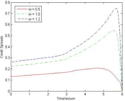
In this subsection, we will illustrate the effect of several parameters including recovery rate, volatility of firm value, the relative price of the firm value and etc. on credit spreads. The credit spreadis defined as the difference between the yields of defaultable bondC and default-free bondZand is given by the following expression:

CS=−lnC−lnZ

T−t .

In the case of exogenous recovery (considered in Theorem 3.2), the credit spread feature is similar with that of [18]. Here we consider the case of endogenous recovery (considered in Theorem 3.3). In this case, the credit spread is differently given in every subinterval.

CSi =−ln

(Ci(V,r,t)/Z(r,t))

T−t =−

ln(ui(V/Z(r,t),t)

T−t , ti ≤ ∀t<ti+1, i=0,· · ·,N−1. (3.14)

LetN=2, t1=3, t2=T=6 (annum)

Basic data for calculation ofCSis as follows: short rate model parameters: a1(t)≡ 0.379∗0.098,a2(t)≡

0.379,sr(t)≡0.077 (Vasicek model); firm value process parameters: dividend rateb=0.05, volatilitysV =1.0;

x = V/Z = 200; correlation of short rate and firm value: ρ = 0.5; λ0 = 0.1,λ1 = 0.3 are respectively

default intensity in the intervals[0,t1],[t1,t2]; K1 = K2 = 100 is default barrier at time t1,t2; recovery rate:

Re =Ru=0.5;α=1/150.

We will analyze(t:CS)plot changing one ofR,sV,ρ,x =V/Z,λandKunder keeping the remainder of data as above.

In what follows, Figure 1 shows that increase of recovery rate results in decrease of credit spread. Figure 2 shows that increase of volatility of firm value results in increase of credit spread. The reason is that when

sV increases, the firm value fluctuates more seriously and there are more risks of default, which results in

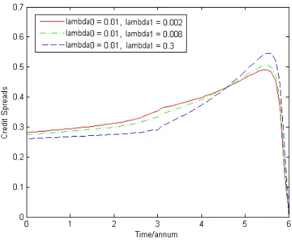
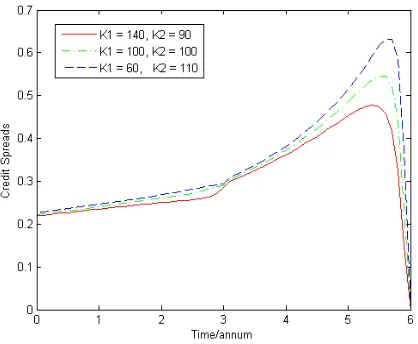
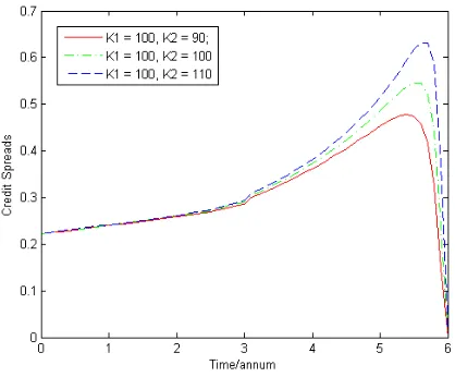
increase of credit spread. Figure 3 shows that increase of correlation between firm value and short rate results in increase of credit spread. Figure 4 shows that increase of firm value results in decrease of credit spread. Figures 5, 6 and 7 show that in the time interval close to the maturity increase of the default intensity results in increase of credit spread but in other time region the circumstance is not so simple. Figures 8, 9 and 10 show that the effect of default barrier on credit spread is different in the time intervals[0,t1]and[t1,T]. The

(9)

Figure 1: Plot(t:CS)whenRe =Ru=0.3, 0.5, 0.8

Figure 2: Plot(t:CS)whensV =0.5, 1.0, 1.2

(10)

Figure 4: Plot(t:CS)whenx=V/Z=180, 220, 260

Figure 5: Plot(t:CS)when(λ0,λ1) = (0.001, 0.002),(0.01, 0.008),(0.1, 0.3)

(11)

Figure 7: Plot(t:CS)when(λ0,λ1) = (0.001, 0.3),(0.01, 0.08),(0.1, 0.002)

Figure 8: Plot(t:CS)when(K1,K2) = (40, 90),(100, 100),(160, 110)

(12)

Figure 10: Plot(t:CS)whenK1=100;K2=90, 100, 110

4

The proofs of the pricing formulae

The proof of Theorem 3.2. Under the assumptions 1)−6), the price model of our bond is given by (3.6). In

(3.6), we use change of numeraire

x=V/Z(r,t), ui(x,t) =Ci(V,r,t)/Z(r,t), ti ≤t<ti+1, i=0,· · · ,N−1. (4.1)

Here Z(r,t)is the price of default free zero coupon bond given by (3.3). If we substitute (4.1) into the first equation of (3.6), note that

Ct=utZ−xuxZt+uZt, VCV =xuxZ, Cr =Zr(u−xux), V2CVV =x2uxxZ,

VCVr=−x2uxxZr, Crr =Zrr(u−xux) +x2uxxZ2r/Z, Zr/Z=−B(t,T)

and consider the equation (3.2) onZ(r,t), then we have

utZ+1

2x

2_u xxZ

h

s2V(t) +2ρsV(t)sr(t)B(t) + (sr(t)B(t))2

i

−bxuxZ−λiuZ+λiRuZ(r,t) =0.

Divide the two hands byZand letS2_X(t) =s2_V(t) +2ρsV(t)·sr(t)·B(t) + (sr(t)B(t))2, then the problem (3.6)

is changed to the following one dimensional problem:



 

 

∂ui

∂t + 1

2S2X(t)x2∂

2_u

i

∂x2 −bx∂

ui

∂x −λi(ui−Ru) =0, ti<t<ti+1, x>0,

ui(x,ti+1) =ui+1(x,ti+1)·1(x >Ki+1) +Re·1(x≤Ki+1), x>0, i=0,· · ·,N−1,

(4.2)

HereuN(x,t)≡1. We use the change of unknown function

ui = (1−Ru)Wi+Ru, (i=0, 1,· · ·,N−1) (4.3)

to have



 

 

∂Wi

∂t + 1

2S2X(t)x2∂

2_W

i

∂x2 −bx∂

Wi

∂x −λiWi =0, ti≤t<ti+1, x>0,

Wi(x,ti+1) =Wi+1(x,ti+1)·1(x>Ki+1) +R1−Rue−Ru ·1(x<Ki+1), x>0, i=0,· · ·,N−1.

(4.4)

HereWN(x,t)≡ 1. Then using thisWi, our bond price is provided by (3.8). The equation (4.4) is called the

equation for the survival probabilityafter the timet∈[ti,ti+1).

(13)

Now we solve the problem (4.4). Wheni=N−1, (4.4) is     

∂WN−1

∂t +

1

2S2X(t)x2

∂2WN−1

∂x2 −bx ∂WN−1

∂x −λN−1WN−1=0, tN−1≤t<tN, x>0,

WN−1(x,tN) =1(x>KN) +Re−Ru1−Ru ·1(x<KN), x>0.

(4.5)

This is a pricing problem of binary options with coefficientsλN−1,λN−1+b,SX(t)whose expiry payoff is a

combination of bond and asset binaries. By the definition of bond binary, we have

WN−1(x,t) =B+KN(x,t;tN;λN−1,λN−1+b,SX(·)) +

Re−Ru

1−Ru

·B−_K

N(x,t;tN;λN−1,λN−1+b,SX(·)), (4.6)

tN−1≤t<tN, x>0.

HereB_Ks(x,t;T;r(·),q(·),σ(·))is given by the formula (2.9) of Theorem 2.1.

For our further purpose, using the relations (2.12) we rewrite (4.6) by the prices of bond and asset binaries with the coefficientsr=0, q=b, σ(t) =SX(t):

WN−1(x,t) =e−λN−1(tN−t)B+_K_N(x,t;tN; 0,b,SX(·)) +

Re−Ru

1−Ru

·e−λN−1(tN−t)_B−

KN(x,t;tN; 0,b,SX(·)), (4.7)

tN−1≤t<tN, x>0.

In order to solve (4.4) wheni =N−2, we need to rewrite (4.6) by the prices of bond and asset binaries with the coefficientsr=λN−2, q=λN−2+b, σ(t) =SX(t)just as noted in the remark 3 in [18].

WN−1(x,t) =e−(λN−1−λN−2)(tN−t)

B_K+_N(x,t;tN;λN−2,λN−2+b,SX(·))

+Re−Ru

1−Ru

·B−_K

N(x,t;tN;λN−2,λN−2+b,SX(·))

, tN−1≤t<tN, x>0. (4.8)

Wheni=N−2 using (4.8), (4.4) is written as follows:                 

∂WN−2

∂t + 1

2S2X(t)x2

∂2WN−2

∂x2 −bx ∂WN−2

∂x −λN−2WN−2=0, tN−2≤t<tN−1, x>0,

WN−2(x,tN−1) =e−(λN−1−λN−2)(tN−tN−1)

h

B+_K

N(x,tN−1;tN;λN−2,λN−2+b,SX(·))·1(x>KN−1) +Re−Ru_1−Ru ·B−_K

N(x,t;tN;λN−2,λN−2+b,SX(·))·1(x>KN−1)

i

+Re_1−Ru−Ru·1(x<KN−1), x>0.

(4.9)

This is a pricing problem of binary options with coefficientsλN−2, λN−2+b, SX(t)whose expiry payoff is a

combination of bond and asset binaries. By the definition of second order binary, we have

WN−2(x,t) =e−(λN−1−λN−2)(tN−tN−1)

B_K+ +

N−1KN(x,t;tN−1;tN;λN−2,λN−2+b,SX(·)) +Re−Ru

1−Ru

·B+_K −

N−1KN(x,t;tN−1;tN;λN−2,λN−2+b,SX(·))

+Re−Ru

1−Ru

·B−_K

N−1(x,t;tN−1;λN−2,λN−2+b,SX(·)), tN−2≤t<tN−1, x>0.

HereBs1s2

K1K2(x,t;T1,T2;r(·),q(·),σ(·))is given by the formula (2.10) of Theorem 2.1.

For our further purpose, using the relations (2.12) we rewriteWN−2(x,t)by the prices of bond and asset

binaries with the coefficientsr=0,q=b,σ(t) =SX(t):

WN−2(x,t) =e−λN−2(tN−1−t)−λN−1(tN−tN−1)B+_K_N₋₁+_K_N(x,t;tN−1;tN; 0,b,SX(·)) +Re−Ru

1−Ru

·he−λN−2(tN−1−t)−λN−1(tN−tN−1)_B+ −

K_N−1KN(x,t;tN−1;tN; 0,b,SX(·)) (4.10) +e−λN−2(tN−1−t)_B−

KN−1(x,t;tN−1; 0,b,SX(·))

i

, tN−2≤t<tN−1, x>0.

(14)

The proof of Theorem 3.3. Under the assumptions 1)−5)0 and 6), the price model of our bond is given by (3.7). In (3.7), we use change of numeraire (4.1), then we have



 

 

∂ui

∂t +

1

2S2X(t)x2∂

2_u

i

∂x2 −bx∂

ui

∂x −λi(ui) +λimin{1,Ruα·x}=0, ti<t<ti+1, x>0,

ui(x,ti+1) =ui+1(x,ti+1)·1{x>Ki+1}+Reα·x·1{x≤Ki+1}, x>0, i=0,· · ·,N−1,

(4.11)

(4.11) is a similar problem with the problem (4.5) in [18]. The only difference is that the (4.11) is a set of terminal value problems for inhomogenous Black-Scholes equations with time dependent coefficients but the (4.5) in [18] is a set of terminal value problems for inhomogenous Black-Scholes equations with constant coefficients. If we follow the way of solving (4.5) in [18] using Theorem 2.1, Lemma 2.2 and the relations (2.12), then we can get the formula (3.13). Then returning to the original variableVand the unknown functionCusing (4.1) we can soon obtain the formula (3.12). The detail is omitted.

5

Conclusions

1) We proved the pricing formula of higher order binary option with time dependent coefficients (Theorem 2.1). This is a generalization of the corresponding results of [7, 15]. Moreover, we generalized the integral formula of higher order binary option on the last expiry date variable into the case with time dependent coefficients (Lemma 2.2).

2) We obtained the pricing formulae of Two factor-model for defaultable bonds with discrete default inten-sity and discrete default barrier in both cases of exogenous and endogenous recoveries (Theorem 3.2 and Theorem 3.3) using the pricing formulae of higher order binary options with time dependent coefficients.

3) In further study the method can seemingly be applied to generalization of the study of [1] into the pricing of defaultable bonds by combining the structural approach and the reduced form approach.

AcknowledgmentsThe authors wish to thank anonymous referees for their comments and suggestions.

References

[1] R. Agliardi, A comprehensive structural model for defaultable fixed-income bonds, Quant. Finance, 11(5)(2011), 749-762.

[2] E. Agliardi and R. Agliardi, Bond pricing under imprecise information,Oper. Res. Int. J., 11(2011), 299-309. [3] E. Agliardi and R. Agliardi, Fuzzy defaultable bonds,Fuzzy Sets and Systems, 160(18)(2009), 2597-2607. [4] R. Agliardi, A comprehensive mathematical approach to exotic option pricing,Math. Methods Appl. Sci.,

35(11)(2012), 1256-1268.

[5] L.V. Ballestra and G. Pacelli, Pricing defaultable bonds: a new model combining structural information with the reduced-form approach, March 11, 2008, Working paper, DOI: 10.2139/ssrn.1492665

[6] Y. Bi and B. Bian, Pricing corporate bonds with both expected and unexpected defaults,Journal of Tongji University (Natural Science), 35(7)(2007), 989-993.

[7] P.W. Buchen, The Pricing of dual-expiry exotics,Quant. Finance, 4(1)(2004), 101-108.

[8] L. Cathcart and L. El-Jahel, Semi-analytical pricing of defaultable bonds in a signaling jump-default model,J. Comput. Finance, 6(3)(2003), 91-108.

[9] L. Cathcart and L. El-Jahel, Pricing defaultable bonds: a middle-way approach between structural and reduced-form models,Quant. Finance, 6(3)(2006), 243-253.

[10] D. Duffie and D. Lando, Term structures of credit spreads with incomplete accounting information,

(15)

[11] J. Ingersoll, Digital contracts: simple tools for pricing complex derivatives,Journal of Business, 73(1)(2000), 67-88.

[12] L. Jiang,Mathematical Models and Methods of Option Pricing, World Scientific, 2005.

[13] H.C. O and N. Wan, Analytical pricing of defaultable bond with stochastic default intensity,Derivatives eJournal, 5(2005), DOI:10.2139/ssrn.723601, arXiv preprint, arXiv:1303.1298[q-fin.PR].

[14] H.C. O, J.J. Jo and C.H. Kim, Pricing corporate defaultable bond using declared firm value,Electronic Journal of Mathematical Analysis and Applications, 2(1)(2014), 1-11.

[15] H.C. O, and M.C. Kim, Higher order binary options and multiple-expiry exotics, Electronic Journal of Mathematical Analysis and Applications, 1(2)(2013), 247-259.

[16] H.C. O, and M.C. Kim, The Pricing of Multiple Expiry Exotics, arXiv preprint, pp 1-16, arXiv:1302.3319[q-fin.PR].

[17] H.C. O, X.M. Ren and N. Wan, Pricing Corporate Defaultable Bond with Fixed Discrete Declaration Time of Firm Value,Derivatives eJournal, 5(2005), DOI: 10.2139/ssrn.723562.

[18] H.C. O, D.H. Kim, S.H. Ri and J.J. Jo, Integrals of Higher Binary Options and Defaultable Bonds with Discrete Default Information, arXiv preprint, arXiv: 1305.6988v4[q-fin.PR].

[19] M. Realdon, Credit risk pricing with both expected and unexpected default,Applied Financial Economics Letters3(4)(2007), 225-230.

[20] P. Wilmott,Derivatives: the Theory and Practice of Financial Engineering, John Wiley & Sons. Inc., 360-583, 1998.

Received: April 25, 2014;Accepted: August 4, 2014

UNIVERSITY PRESS