Forestry & Natural-Resource Sciences Last Correction: Sep. 31, 2017
INCORPORATING A LOCAL-STATISTICS-BASED SPATIAL
WEIGHT MATRIX INTO A SPATIAL REGRESSION MODEL TO
MAP THE DISTRIBUTION OF NON-NATIVE INVASIVE
ROSA
MULTIFLORA
IN THE UPPER MIDWEST
Weiming Yu
1, Zhaofei Fan
2∗, W Keith Moser
3 1Department of Forestry, Mississippi State University, Starkville, MS, USA
2∗
Cor. Author, School of Forestry and Wildlife Sciences, Auburn University, Auburn, AL, USA
3USDA Forest Service, Rocky Mountain Research Station, Fort Collins, CO, USA
Abstract.In this study, we extended the spatial weight matrix defined by Getis and Aldstadt (2004) to a more general case to map the distribution ofRosa multiflora, an invasive shrub, across the Upper Midwest counties in a spatial lag model (SLM) context. Both the simulation study and the application to the invasion data of invasiveRosa multiflora collected in 2005–2006 proved that the modified spatial weight matrix outperforms its original case and the contiguity- and nearest distance- based spatial weight matrices in diagnostic statistics and resultant invasion maps. The geographical distribution of Rosa multiflora in the Upper Midwest was significantly associated with latitude; local clusters (groups of counties) of high abundance/presence ofRosa multiflorawere significantly determined by TRPF (a ratio of road density to percentage of forest cover at the county level), a variable reflecting the intensity of human disturbance. Both the multiple linear regression model and the SLM models with the original spatial weight matrix and contiguity- and nearest distance- based spatial weight matrices incorporated tended to underestimate the effect of forest type (community) on multiflora rose. As a conclusion, the SLM model incorporating the modified spatial weight matrix has potential applications in mapping spatial data with strong clustering patterns and estimating spatial autocorrelation structure and covariate effects in ecological studies.
Keywords: invasive plants, local spatial statistics, spatial autocorrelation, spatial weight matrix
1
Introduction
The invasion and spread of non-native invasive plants (NNIPs) into natural systems is an ecological phe-nomenon characterized by spatial autocorrelation across a set of spatial scales and organizational levels (Vermeij 1996). Application of spatial models to map patterns of NNIPs and to quantify contributing factors is of theoreti-cal and applied importance to the monitoring and control of NNIPs. Spatial weight matrices have been used in regression models to account for autocorrelation in data for scientific inferences (e.g., Legendre 1993, Fortin et al. 2006, Kissling and Carl 2008, Zhang et al. 2005, 2009, Lu and Zhang 2010, 2011). Essentially, the purpose of spatial weight matrices is to define the spatial autocor-relation structure of underlying bioecological processes such as the spread of NNIPs across a landscape. Mis-specification of spatial autocorrelation usually has two consequences:
1. the estimation of coefficient variances has a down-ward bias, which results in an inflated type-I error and incorrect inferences; and
2. the estimation of parameters in statistical models is incorrect and results in the wrong interpretation of the environmental variables (Anselin and Bera 1998, Keitt et al. 2002, Haining 2003).
Thus, the choice of a spatial weight matrix is critical for spatial regression models.
It is still a challenge as there are no specific guidelines or schemes for the selection of spatial weight matrices. Stakhovych and Bijmolt (2009) summarized the litera-ture concerning the choice of spatial weight matrices into three avenues of investigation. First, the most popular approach is distance- or neighborhood-related, such as spatial contiguity, inverse distance raised to a certain power,n-nearest neighbors, share of common boundaries, ranked distance, and centroids (Anselin and Bera 1998,
Copyright©2017 Publisher of theMathematical and Computational Forestry & Natural-Resource Sciences
Waller and Gotway 2004). Anselin (1988) argued that spatial weight matrices should be exogenous and should be based on theoretical assumptions on the spatial struc-ture. However, this approach has its limitations: the spatial weight matrix may not reflect the real spatial structure; and specification of the matrix is model-based. Second, specification of spatial weight matrices is model-based. LeSage and Parent (2007) and Holloway and La-par (2007) used the Bayesian model to choose the spatial weight matrix. Kostov (2010) used the component-wise model boosting algorithm (Buhlmann 2006) when deal-ing with the selection of spatial weight matrices. The limitation of the model-based approach is the large num-ber of potential spatial weight matrices and relatively limited computational capability, especially when the number of observations is large. Third, specification of spatial weight matrices is data-driven. Researchers con-struct spatial weight matrices based on the extracted information about the spatial relationships from existing data (Getis and Aldstadt 2004). Getis and Aldstadt (2004) constructed a spatial weight matrix by using the local spatial statistic Getis-Ord G∗i(d). Subsequently, Aldstadt and Getis (2006) used a sophisticated algorithm to construct a spatial weight matrix that depended on the local spatial statistic Getis-OrdG∗i and identified the shape of spatial clusters.
Getis and Aldstadt (2004) found that the spatial weight matrix based on the local spatial statistic performs better than spatial weight matrices based on contiguity, inverse distance, or semi-variance model according to the Akaike Information Criterion (AIC) (Akaike 1974). They at-tributed these results to the local adaptive nature of this spatial weight matrix. However, this weight matrix is not directly related to the distance even though the local spatial statistic Getis-Ord G∗i(d) is implicitly re-lated to the distance. According to Tobler’s first law (Tobler 1970), the inverse distance is used to weight the
local spatial statisticG∗
i(d) in this study such that the
modified spatial weight matrix is explicitly related to the distance while maintaining its local adaptive nature. Then a natural and immediate question is: Which matrix will perform best?
The major objective of this study is 1) to modify the spatial weight matrix defined by Getis and Aldstadt (2004), and compare the performance of the modified spatial weight matrix and its original case through a simulation study; and 2) compare the performance of the original and modified (local-statistics based) spatial weight matrix with the commonly used contiguity- based and nearest distance-based spatial weight matrix through an application to field data to map the distribution of Rosa multiflora, a major non-native invasive shrub, in the Upper Midwest states. In addition, this study will explore the effect of incorporated spatial weight matrices
on covariate selection and interpretation through com-parison of the derived spatial regression models and a multiple linear regression model, a reference model that does not incorporate a spatial weight matrix.
2
Definition of Getis-Ord
G
∗i(
d
)
Getis and Ord (1992) and Ord and Getis (1995) intro-duced the spatial statisticsG(d),Gi(d) andG∗i(d). G(d)
is a global indicator of spatial clustering; butGi(d) and G∗i(d) can be used to detect local clusters. These three statistics are defined as,
G(d) =
P
i
P
jwij(d)xixj
P
i
P
jxixj
, (1)
Gi(d) =
P
j(wij(d)xj−Wix¯(i)) s(i){[(nS1i)−W
2
i]/(n−2)}1/2
, j6=i,and
(2)
G∗i(d) =
P
j(wij(d)xj−Wi∗x¯) s∗ {[(nS∗
1i)−W
∗2
i ]/(n−1)}1/2
, all j (3)
Where,wij(d) is a symmetric 0 or 1 spatial weight
ma-trix with 1 for all links defined as being within dis-tancedof theith observation; W
i =P j6=i
wij(d), Wi∗=
Wi+wii, S1i =Pjw 2
ij, j6=i,andS1∗i=
P
jw 2
ij; ¯x(i) = P
jxj (n−1), ands
2(i) = P
jx 2 j
(n−1)−(¯x(i))
2, j6=i; ¯xands2denote
the usual sample mean and variance, respectively. A positive value of G∗i(d) indicates a cluster of rel-atively high values within d of the ith observation; a
negative value ofG∗i(d) indicates a cluster of relatively low values withindof theithobservation. The difference
between Gi(d) and G∗i(d) is that the former does not
consider the contribution of theith observation, but the
latter does.
2.1 Constructing spatial weight matrices using
Getis-Ord G∗i(d) In general, G∗i(d) values monotoni-cally increase around theith observation as the distance from that observation increases up to a point, then begin to decrease. This point is defined as the critical distance,
dc,(Getis and Aldstadt 2004), where any continuity in
spatial dependence or association over distance ends; thus, it defines the cluster diameter (Getis and Aldstadt 2004). To computeG∗i(d), we need to define the neigh-bors of theith observation. Getis and Aldstadt (2004)
calculated dc based on one unit separating centers of
rook’s case neighbors – the neighbors share a common boundary – within the distancedc. For simplicity, in this
study, we use all neighbors withindc. We also denoted1
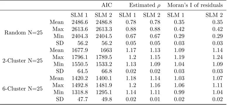
Table 1: Results of simulation study, where SLM 1 uses the spatial weight matrix W∗and SLM 2 uses the modified spatial weight matrixW ∗ ∗.
AIC Estimatedρ Moran’s I of residuals
SLM 1 SLM 2 SLM 1 SLM 2 SLM 1 SLM 2
Random N=25
Mean 2486.6 2486.8 0.78 0.78 0.35 0.35
Max 2613.6 2613.3 0.88 0.88 0.42 0.42
Min 2404.3 2404.5 0.67 0.67 0.29 0.29
SD 56.2 56.2 0.05 0.05 0.03 0.03
2-Cluster N=25
Mean 1677.9 1663 1.17 1.13 1.09 1.14
Max 1796.1 1789.5 1.2 1.15 1.19 1.24
Min 1550.5 1533.2 1.13 1.09 1.04 1.09
SD 64.5 66.8 0.02 0.02 0.03 0.03
6-Cluster N=25
Mean 1420.2 1400.1 1.18 1.14 1.03 1.07
Max 1492.8 1481.9 1.2 1.16 1.06 1.11
Min 1318.8 1295.1 1.14 1.11 0.99 1.04
SD 47.7 49.8 0.02 0.01 0.02 0.02
and Aldstadt (2004) defined the spatial weight matrix
W∗ as,
1. Whendc= 0,
w∗ij = 0, for allj
2. Whendc=d1, w∗
ij = 1, for allj, wheredij =dc; wij∗ = 0, otherwise;
3. Whendc> d1,
lwij∗ =|G
∗
i(dc)−G∗i(dij)| |G∗i(dc)−G∗i(0)|
, for alljwheredij ≤dc;
w∗
ij = 0, otherwise. (4)
Where, G∗i(dc) is the Gi∗ score at dc, and G∗i(0) is
the G∗i score for theith observation only andG∗i(0) is the base from to which other measures of G∗
i(d) are
compared. According to the definition, wij∗ is 0 for all the observations that have no spatial correlation with its neighbors, including thatdc is equal to 0 or the distance
between theith andjth observation is greater thand c.
According to the definition of Getis-OrdGi∗(d), the
distance (d) identifies which observations should be in-cluded in the calculation, and the statistic Gi∗(d) is
implicitly related to the distance. Thus,W∗is implicitly related to the distance. However, Carl and K¨uhn (2007) argued that the similarity of the values of two observa-tions is inversely related to the geographical distance between each other. In other words, we should assign greater weights to the observations closer to the given observations and smaller weights to the observations that
are farther away from the given observations. There-fore, in this study we used inverse-distance to weight the Getis–OrdGi∗(d) in order to obtain a modified spatial
weight matrix W∗∗ such that it explicitly reflects the impact of distance and meanwhile maintains the local adaptive nature ofW∗, thereby outperforming the other spatial weight matrices. The modified spatial weight matrixW∗∗ is defined as,
1. Whendc= 0,
wij∗ = 0, for allj
2. Whendc=d1,
w∗
ij = 1, for allj, wheredij =dc; wij∗ = 0, otherwise;
3. Whendc >d1,
lwij∗ =
G
∗
i(dc)/dkc−G∗i(dij)/dkij
G∗i(dc)/dkc −G∗i(0)
, for alljwhere :
dij ≤dc;
wij∗ = 0, otherwise. (5)
Where,kis a non-negative constant. For simplicity, in this study,kis set to one.
The Spatial Lag Model (SLM) was used in the simula-tion study as follows:
Y =α+ρW Y +βX+ε, (6)
whereY is the response variable generated by the simula-tion,ρrepresents the dependence structure of the variable
spatial weight matrix (W∗orW∗∗). Just as in Getis and Aldstadt (2004), we added a dummy variableX, which takes on the value of one for all observations having no dependence structure and zero otherwise, to compensate for the zero-rows effects in W. The parameters were estimated by using maximum-likelihood methods.
2.2 Simulation design For the simulation study, we
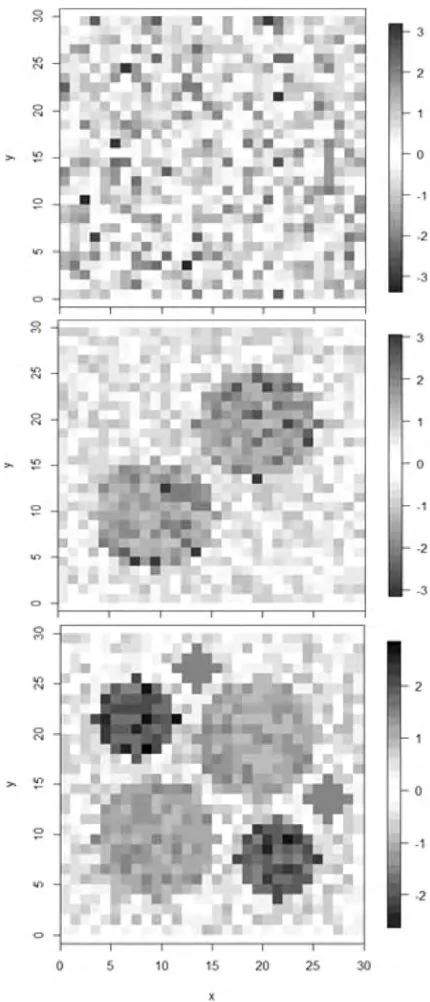
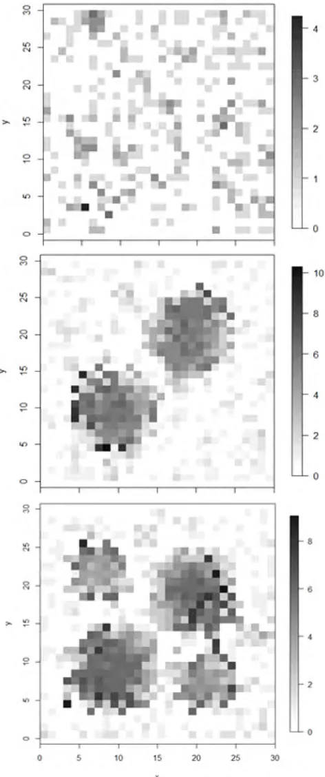
used the same design as Getis and Aldstadt (2004) except that we changed the cluster radius in the 2-cluster case to 6 instead of 8 to avoid overlap of cells (Table 1). Each of three types of 30 by 30 raster data sets was simulated for 25 times. The 25 replications with cluster patterns were considered to be sufficient for representing a wide variety of spatial structures (Getis and Aldstadt 2004). The three types are a random normal representing a pattern with no spatial autocorrelation among the values placed in the cells, a pattern of 2 clusters of equal sizes, and a pattern of 6 clusters indicating the spatial structure with random combinations of multiple patches of varying sizes. All the values put in the cells were generated from a standard normal distribution. Figure 1 shows one realization of the random normal pattern, 2-cluster pattern, and 6-cluster pattern representing the potential spatial structure of collected data such as the distribution of invasive shrubs per se. For the data sets shown in Figure 1, Figure 2 shows the spatial distribution of the critical distances, which determine the size of spatial weights. For theith observations, the critical distance
is calculated as follows: first, for each givend, we found the nearest neighbors of theith observations within d; second, we calculated theG∗i(d); last, dc is defined as
the valuedsuch that G∗i(d) is the maximum andG∗i(d) is monotonically increasing in the interval (0, d).
2.3 Evaluation criteria Per Getis and Aldstadt
(2004), AIC, autocorrelation coefficientρ, and Moran’s I of residuals were used to evaluate the model performance. Given a set of candidate models for the data, the model with a minimum AIC value will be chosen. AIC penal-izes the model with more parameters since the value of AIC increases as the number of parameters in the model increases.
Getis and Aldstadt (2004, page 98) argued that “the autocorrelation coefficient gives an interpretation for the possible association between WY andY”. Ifρ= 1, it means that W is a good representation of the spatial autocorrelation among data; otherwise, ifρ is close to 0, it means thatW is not a good representation of the spatial autocorrelation among data. In addition, Getis and Aldstadt (2004) used Moran’s I to detect the spatial autocorrelation among the residuals. The Moran’s I is
Figure 2: Critical distance (dc) for the random pattern (a), 2-cluster pattern (b), and 6-cluster pattern (c) cor-responding to the data sets in Figure 1. Distances are based on nearest neighbors.
defined as,
I=
N∗ N
P
i=1 N
P
j=1
wij(ei−¯e)(ej−e¯)
N
P
i=1 N
P
j=1 wij∗
N
P
i=1
(ei−e¯)
(7)
where,N is the number of cells,eis the residuals vector, andwij is a spatial weight between theithobservation
andjthobservation. IfW accounts for all of the spatial variation iny, the residuals should be spatially random. Moran’s I of the residuals was computed by using the sameW that was used in the corresponding candidate models.
An applied example with non-native invasive plant data
Data on non-native invasive plants in forested ecosys-tems were collected from seven states in the Upper Mid-west: Indiana, Illinois, Iowa, Missouri, Michigan, Wiscon-sin, and Minnesota. Of these states, northern Minnesota, northern Wisconsin, northern Michigan, and southern Missouri are the most heavily forested areas (forested lands>30%), while the middle of this region, covered mostly by prairie prior to European-American settlement, is currently a mosaic of agricultural lands and urban ar-eas (forested lands ˜10%). Extensive human activities (e.g., timber harvesting, clearing land for settlement) in the Upper Midwest created many opportunities for the establishment and spread of NNIPs.
During the 2005–2006 inventory years, 8, 662 U.S. De-partment of Agriculture, Forest Service, Forest Inventory and Analysis (FIA) phase 2 plots in the seven states were assessed for presence or absence and cover (percentage of total plot area) of any of the 25 non-native invasive plant species (Fan et al. 2013). In total, 594 of 649 counties in the Upper Midwest have FIA plots on forest land and 2, 039 (23.5) of 8, 662 FIA plots were invaded by one or more of these invasive shrubs. Among the assessed NNIPs, multiflora rose (Rosa multiflora Thunb., MFR hereafter) was most prevalent and was present in 1, 320 (15.2% of all FIA plots).
Mapping the distributional pattern of MFR at the county level
In this data set, the average number of forested FIA plots per county is 14, but varies dramatically by county and subsequently may affect the estimation of the abun-dance (presence probability) of MFR. To overcome this potential bias from the sample size, one common way is using the nearest neighbor (moving window) method to adjust the abundance of MFR in a county as:
Abundancei=
P
j∈ηi sj
P
j∈ηi nj
Where, sj is the number of the presence plots in the
county j, nj is the total plots in the county j, and ηi
is the set of counties that share a boundary with the countyi, including the countyi. However, because this study is not for predictive purposes, but instead for understanding how different spatial weight matrices work in mapping the distributional pattern of MFR, we ignore the sample size effect. The presence probability of MFR in a county was calculated as the ratio of the number of presence plots to the total number of FIA plots and was assigned a value of zero if no FIA plots were installed in a county. An arcsine transformation was conducted on the presence probability of MFR, and the transformed presence probability was used as the response variable in spatial mapping through regression models.
Based on the literature and exploratory data analyses (Fan et al. 2013), the following covariates were selected to model the abundance of MFR (equation (4)): percentage of forest cover as a whole or by major forest-type group at the county level, road (interstate and state highway) den-sity, and latitude/longitude (using the geometric center of each county). The forest cover type map layer was down-loaded from the National Atlas (www.nationalatlas.gov). Twenty-five forest cover types were obtained from the Advanced Very High Resolution Radiometer (AVHRR) and Landsat Thematic Mapper (TM) imagery. We combined these forest cover types into 7 forest-type groups:conifer, oak/pine, oak/hickory, oak/gum/cypress, elm/ash/cottonwood, maple/beech/aspen/birch,and non-forest. Their percentage areas (ratio of each forest cover type to area of each county, %) and total forest percent cover were calculated by using GIS for each Upper Mid-west county. The road map layer was obtained from the National Atlas (www.nationalatlas.gov) and road densi-ties (the length of interstate and state highway per unit area, km/km2) were calculated for all Upper Midwest counties by using Spatial Analyst in ArcGIS. Further-more, we defined a new variable, RDPF, as the ratio of the road density and the county forest percentage. We found that RDPF better describes the intensity of human disturbances and forest fragmentation and is more closely correlated with the abundance of invasive shrubs than either road density or county forest percent-age alone.
Overall, abundance of MFR changed linearly with the covariates except for latitude. To reflect the “mound” shaped relationship between abundance and lati-tude/longitude, the quadratic form of latitude/longitude was included in the process of model construction. We used a multiple linear regression model (MLR, neglecting spatial autocorrelation, used to compare with the SLM) and SLM in equation (4) (SLM, the original and modi-fied spatial weight matrix, one contiguity (queen’s rule)-based spatial weight matrix and onek-nearest [k= 3]
distance-based spatial weight matrix incorporated to ac-count for spatial autocorrelation) to map the change of abundance of multiflora rose with the selected covariates. Here, Y is the arcsine transformed abundance of MFR; X is a set of covariates consisting of: latitude (quadratic form), forest percentage as a whole and by forest-type groups (conifer, oak/pine, oak/hickory, oak/gum/cypress, elm/ash/cottonwood, maple/aspen/beech/birch), road density, and TRPF; βis are the regression coefficients
to be estimated;ν is the independent error vector and assumed to be normally distributed;ρis the simultane-ous autoregressive error coefficient; andW is the spatial weight matrix. SLM 1 and SLM 2 usedW∗ as defined by Getis and Aldstadt (2004) and the modifiedW∗∗, re-spectively; and SLMs 3 and 4 used the contiguity-based spatial weight matrix and the nearest distance-based spatial weight matrix, respectively. AIC was used to select the best model from the candidates. Further, to assess the goodness-of-fit of both SLMs, we reported the Nagelkerke pseudo-R2, which is defined as:
R2= 1−(L(Mintercept)/L(Mf ull)
2/N
1−(L(Mintercept))2/N
(9)
where Mf ull is the model with predictors, Mintercept
is the model without predictors, L(.) is the likelihood of the corresponding models, and N is the number of observations. We also evaluated the spatial patterns of residuals by using local Moran’s I.
All statistical computation, analysis, and simulation were conducted under the R statistical environment (R Development Core Team 2011). The packagespdep was used to fit the SLM model and thespandmaps packages were used to draw graphics (Bivand et al. 2008).
2.4 Results and Discussion The simulation results
showed that for all cases, the value of the autocorrelation coefficient,ρ, is significantly different from 0 (p<0.0001) (Table 1). In general, the range of Moran’s I is in the interval (-1, 1). In the 2- and 6-cluster cases, however, Moran’s I values were slightly greater than 1. This result may have occurred because the number N in equation (7) does not represent the actual number of cells as some observations have no spatial autocorrelation with their neighbors and the corresponding rows in the modified spatial weight matrices are zero.
I
·
8
,,
2
0
38
-9 -9
..
9
·
.
-
9
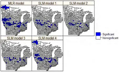
Figure 4: Spatial clusters of residuals of the MLR and SLM models at the significant level of alpha = 0.05. SLM model 2 and model 3 are best for they have fewest and smallest clusters.
models in both the 2- and 6-cluster cases. Thus, we conclude thatW∗∗ performs better thanW∗ according to the AIC rule when spatial autocorrelation occurred in the data.
Equation (5) can be rewritten as:
w∗∗ ij =
G∗i(dc)−G∗i(dij)×dc/dij
|G∗i(dc)−G∗i(0)×dc|
(10)
In general, ifdij is close todc (i.e.,dc/dij is close to 1),
thenw∗∗ij is greater thanwij∗. If dij is much smaller than dc (i.e.,dc/dij is large enough), thenw∗∗ij is smaller than w∗ij. Thus, the modification of W∗ adjusts weights by assigning a greater weight to observations that are far away from ith observations and assigning smaller
weights to observations close to ith observations. The
better performance of the modified spatial weight matrix may be attributed to the fact that the original case
W∗ over-weighted the observations that are close toith
observations and under-weighted the observations that are far away fromith observations (Carl and K¨uhn 2007).
Notice thatW∗is a special case of W∗∗ ask= 0, and
W∗∗ extends W∗ to a more general case without losing its local adaptive property. On the other hand, though
kis set to one for simplicity, we may choose an optimal
k, which minimizes AIC, by using the trial-and-error method with the data.
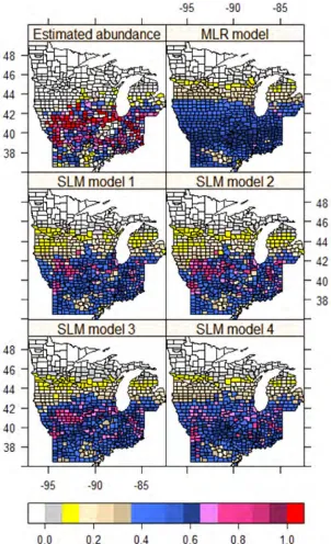
The spatial distribution of MFR at the county level showed a strong spatial autocorrelation characterized by several clusters centered in southern Iowa, northeastern Illinois, and north-central Indiana (Figure 3). The SLMs, to varying degrees, captured major clusters; the MLR model, however, failed to distinguish these clusters (Fig-ure 3). Among the SLMs, model 2, which was based on the modified spatial weight matrix (W∗∗), had the smallest AIC and MSE and largest Nagelkerke
pseudo-R2 (Table 2). The spatial patterns of residuals showed that SLM 2 was comparable to SLM 3 (which used the contiguity-based spatial weight matrix), but better than the MLR model and the original Getis-OrdG∗
i(d) local
statistic and nearest-distance-based SLMs (1 and 4) in terms of fewer and smaller clusters of residuals (Figure 4). A closer county-by-county inspection indicated that the abundance indicated by SLM 2 is larger in most counties in the central and southern parts of the study region, but smaller in the northern portion than for other SLMs. The difference in AIC, MSE, and Nagelkerke pseudo-R2
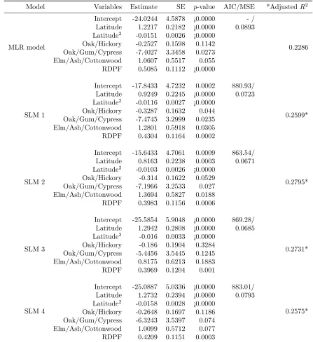
Table 2: The results of multiple linear regression (MLR) model and four spatial lag models (SLMs) to map the presence probability of multiflora rose in the Upper Midwest counties.
Model Variables Estimate SE p-value AIC/MSE *AdjustedR2
MLR model
Intercept -24.0244 4.5878 ¡0.0000 - /
0.2286
Latitude 1.2217 0.2182 ¡0.0000 0.0893
Latitude2 -0.0151 0.0026 ¡0.0000
Oak/Hickory -0.2527 0.1598 0.1142
Oak/Gum/Cypress -7.4027 3.3458 0.0273
Elm/Ash/Cottonwood 1.0607 0.5517 0.055
RDPF 0.5085 0.1112 ¡0.0000
SLM 1
Intercept -17.8433 4.7232 0.0002 880.93/
0.2599*
Latitude 0.9249 0.2245 ¡0.0000 0.0723
Latitude2 -0.0116 0.0027 ¡0.0000
Oak/Hickory -0.3287 0.1632 0.044
Oak/Gum/Cypress -7.4745 3.2999 0.0235
Elm/Ash/Cottonwood 1.2801 0.5918 0.0305
RDPF 0.4304 0.1164 0.0002
SLM 2
Intercept -15.6433 4.7061 0.0009 863.54/
0.2795*
Latitude 0.8163 0.2238 0.0003 0.0671
Latitude2 -0.0103 0.0026 ¡0.0000
Oak/Hickory -0.314 0.1622 0.0529
Oak/Gum/Cypress -7.1966 3.2533 0.027
Elm/Ash/Cottonwood 1.3694 0.5827 0.0188
RDPF 0.3983 0.1156 0.0006
SLM 3
Intercept -25.5854 5.9048 ¡0.0000 869.28/
0.2731*
Latitude 1.2942 0.2808 ¡0.0000 0.0685
Latitude2 -0.016 0.0033 ¡0.0000
Oak/Hickory -0.186 0.1904 0.3284
Oak/Gum/Cypress -5.4456 3.5445 0.1245
Elm/Ash/Cottonwood 0.8175 0.6213 0.1883
RDPF 0.3969 0.1204 0.001
SLM 4
Intercept -25.0887 5.0336 ¡0.0000 883.01/
0.2575*
Latitude 1.2732 0.2394 ¡0.0000 0.0793
Latitude2 -0.0158 0.0028 ¡0.0000
Oak/Hickory -0.2648 0.1697 0.1186
Oak/Gum/Cypress -6.3243 3.5397 0.074
Elm/Ash/Cottonwood 1.0099 0.5712 0.077
RDPF 0.4209 0.1151 0.0003
*Nagelkerke pseudo-R2; SLM 1 and 2 use the original and modified Getis-Ord G∗i based spatial weight matrix,
al. (2013) mapped the abundance of invasive shrubs and analyzed the associated factors by using the nonpara-metric kernel smoothing and CART (classification and regression tree), respectively. Invasive shrubs such as MFR were predominantly distributed in the central part of the study area with two major clusters surrounding Chicago, Illinois and Des Moines, Iowa, similar to the simulated 2-cluster pattern. Test statistics indicate that SLM 2 performed well; simulated data conformed well to actual data.
With the model per se, the estimated regression coeffi-cient for RDPF in the SLMs were significantly smaller than that in the MLR model, suggesting that RDPF had less leverage in predicting the abundance of MFR after the spatial autocorrelation was partially interpreted by the spatial weight matrix (Table 2). There was no signif-icant difference in the estimated RDPF among the four SLMs although the estimated values for models 2 and 3 tended to be small compared to models 1 and 4.The estimated regression coefficients for other covariates in models 3 and 4 were nearly identical to those in the MLR model. However, models 1 and 2 had significantly larger estimated values for the intercept and smaller estimated values for latitude (linear term) than the MLR model and SLMs 3 and 4. Further, forest type covariates were statistically significant in models 1 and 2 in contrast with the marginal significance or non-significance in the MRL model and models 3 and 4. The MLR model, as a benchmark, did not account for spatial autocorrela-tion, which resulted in inaccurate parameter estimation and invasive shrub simulation because of the downward bias in the estimation of coefficient variances (Anselin and Bera 1998, Keitt et al. 2002, Haining 2003). The SLMs with the contiguity-based spatial weight matrix (model 3) and the nearest distance-based spatial weight matrix (model 4) may somewhat improve the estimates for certain covariates (e.g., RDPF). But the SLMs with the local statistics-based spatial weight matrix perform better in mapping the regional patterns of clustered MFR data and estimating covariate effects (Table 2).
Compared to the original Getis-OrdG∗i(d)-based spa-tial weight matrix (in SLM 1), the modified spaspa-tial weight matrix (in SLM 2) renders a relatively large effect for the intercept, forest types, and the quadratic term of latitude, but a small effect for RDPF and latitude. This result means that the modified spatial weight matrix explained more spatial variation (clusters) related to lat-itude and forest types than the original spatial weight matrix as shown by the spatial pattern of residuals (Fig-ure 4). The significant association (p <0.0003) between abundance of MFR and latitude (including its quadratic form) reflected the unimodal distribution pattern in the latitudinal direction (from south to north) with major clusters of high presence probability centered in southern
Iowa, northern Missouri, and northern Illinois (Figure 3). The abrupt decrease of invasive shrubs at latitudes greater than 44°N may suggest that the dispersal of MFR, which is the most prominent of the major invasive shrubs, is limited by the extremely low temperatures in the northern part of the region (Doll 2006, Denight et al. 2008).
The abundance of MFR was negatively associ-ated with the forest-type groups oak/hickory and oak/gum/cypress, and positively related to the forest-type group elm/ash/cottonwood in all models. This relationship indicated that MFR were more likely to in-vade counties with higher proportions of lowland forests such as elm/ash/cottonwood. MFR was less abundant in bottomland forests (e.g., oak/gum/cypress) or upland forests (e.g., oak/hickory), a result consistent with the traits of the major invasive shrubs (e.g., non-native bush honeysuckles). MFR is most productive in sunny areas with well-drained moist uplands and lowlands; it endures shade, sun, and damp or dry conditions, but does not grow well in standing water or in extremely dry areas (Bowman’s Hill Wildflower Preserve 1997, Munger 2002, Doll 2006). The appearance of these three forest-type groups in the MLR and SLM models in predicting the abundance of MFR most likely reflected their prominence (e.g., oak/hickory, elm/ash/cottonwood) in the area (i.e., Iowa, Missouri, Illinois, and Indiana) where IPs were widely distributed (Moser et al. 2016).
disturbances. The significant (p < 0.001), positive as-sociation between the abundance of MFR and RDPF confirms human disturbance as one of the major driving factors for its invasion and spread in the Upper Midwest. Greater human presence reduces native forest ecosystem defenses, by upsetting ecological stability via disturbance and increasing the opportunity for niche capture by inva-sive plants, and often increases propagule pressure, both passively and actively, thus further increasing abundance of the invaders (Macdonald 1994, Pimentel et al. 2005, Richardson and Pysek 2006).
3
Conclusions
In this study, we compared the performance of two spatial weight matrices, W∗ and W∗∗, based on the local spatial statistics Getis-Ord G∗i. We found that with strong spatial autocorrelation of invasive plants such as multiflora rose W∗∗ performs better than W∗
and the contiguity- and nearest distance-based spatial weight matrix. The spatial weight matrixW∗ is a special case of the spatial weight matrix W∗∗. The modified spatial weight matrix W∗∗ extends the spatial weight matrix W∗ to a more general case without losing its local adaptive property. The SLM with a spatial weight matrix based on local spatial statistics such as Getis-OrdG∗i provides a promising approach to map regional patterns of sophisticated ecological phenomena such as the invasion and spread of invasive plants. Compared to spatial weight matrices defined through global statistics such as geostatistical or inverse-distance models, the local statistics-based spatial weight matrix demonstrates its strength and efficacy in explaining the spatial variation of the data, particularly when the distribution of invasive plants is controlled by a number of multi-scale processes and takes a spatial pattern of multiple clusters of various sizes.
Our results also indicated that spatial weight matrices might affect the choice of the factors used to explain the abundance of invasive plants. In addition to spatial autocorrelation, which was explained by spatial weight matrices, the variation in abundance of invasive plants such as multiflora rose in the Upper Midwest counties was attributable to human disturbances (RDPF), a geo-graphic factor (latitude), and forest conditions. But the significance of these factors in the model may change with the choice of spatial weight matrices. In this study, with the original and modified spatial weight matrix based on the local spatial statistics Getis-OrdG∗i, county-level proportions of oak/hickory, oak/gum/cypress, and elm/ash/cottonwood forest-type groups became signif-icant at the significance level of α = 0.05 compared to the marginal significance or non-significance with the MLR model and the SLMs with contiguity- and
distance-based spatial weight matrix. The distribution of multi-flora rose was primarily related to latitude and human disturbance, but forest types were also related to the observed clustering patterns. The SLM with the modi-fied spatial weight matrix performs better in explaining the spatial patterns of multiflora rose and detecting sec-ondary covariate effects than the MLR model and the SLMs with spatial weight matrices based on the original Getis-OrdG∗i contiguity, or distance.
References
Akaike, H. 1974. A new look at the statistical model iden-tification.IEEE Transactions on Automatic Control. 19(4): 716–723.
Aldstadt, J., and A. Getis. 2006. Using AMOEBA to create a spatial weights matrix and identify spatial clusters.Geographical Analysis. 38: 327–343.
Anselin, L. 1988. Spatial Econometrics: Method and Models. the Netherlands: Kluwer Academic Publishers.
Anselin, L., and A. Bera. 1998. Spatial dependence in linear regression models with an introduction to spa-tial econometrics. InHandbook of Applied Economic Statistics, Ullah. A. (ed.). Marcel Dekker, New York.
Bivand, R. S., E. J. Pebesma, and V. Gomez-Rubio. 2008. Applied Spatial Data Analysis with R. Springer, New York.
Bowman’s Hill Wildflower Preserve (BHWP). 1997. Multiflora rose - invasive exotics. Available online at: www.bhwp.org/cms/files/file ID96816.pdf; last ac-cessed: Sept. 29, 2011.
Buhlmann, P. 2006. Boosting for high-dimensional linear models.The Annals of Statistics. 34(2): 559–583.
Carl, G., and I. K¨uhn. 2007. Analyzing spatial autocor-relation in species distributions using Gaussian and Logit models.Ecological Modelling. 207(2-4): 159–170.
Denight, M. L., P. J. Guertin, D. L. Gebhart, and L. Nelson. 2008. Invasive Species Biol-ogy, Control, and Research, Part 2: Multiflora Rose (Rosa Multiflora). Available online at www.cecer.army.mil/techreports/ERDC TR-08-11/ERDC TR-08-11.pdf; last accessed Sept. 29, 2011.
Doll, J. D. 2006. Biology of Multiflora Rose.
P. 239 in North Central Weed Science
Society Proceedings. Available online at
Fan, Z., W. K. Moser, M. H. Hansen, and M. D. Nelson. 2013. Regional patterns of major non-native invasive plants and associated factors in Upper Midwest forests. Forest Science.59 (1): 38–49.
Fortin, M.J., M.R.T. Dale, and J. Hoef. 2006. Spatial analysis in ecology.Encyclopedia of Environmetrics.4: 2051–2058.
Gelbard, J. L. and J. Belnap. 2003. Roads as conduits for exotic plant invasions in a semiarid landscape. Con-servation Biology. 17(2): 420–432.
Getis, A., and J. K. Ord. 1992. The analysis of spatial association by use of distance statistics.Geographical Analysis. 24(3): 189–206.
Getis, A., and J. Aldstadt. 2004. Constructing the spatial weights matrix using a local statistic. Geographical Analysis. 36(2): 90–104.
Haining, R. P. 2003. Spatial Data Analysis: Theory and Practice. Cambridge University Press, Cambridge, United Kingdom.
Holloway, G., and M. L. A. Lapar. 2007. How big is your neighborhood? Spatial implications of market participation among Filipino smallholders.Journal of Agricultural Economics. 58(1): 37–60.
Keitt, T. H., O. N. Bjørnstad, P. M. Dixon, and S. Citron-Pousty. 2002. Accounting for spatial pattern when mod-eling organism-environment interactions. Ecography. 25(5): 616–625.
Kissling, W. D., and G. Carl. 2008. Spatial autocorrela-tion and the selecautocorrela-tion of simultaneous autoregressive models.Global Ecology and Biogeography. 17(1): 59– 71.
Kostov, P. 2010. Model boosting for spatial weighting matrix selection in spatial lag models.Environment and Planning B: Planning and Design. 37(3): 533–549.
Legendre, P. 1993. Spatial autocorrelation: Trouble or new paradigm? Ecology. 74(4): 1659–1673.
LeSage, J. P., and O. Parent. 2007. Bayesian model averaging for spatial econometric models.Geographical Analysis. 39(3): 241–267.
Lu, J., and L. Zhang. 2010. Evaluation of parameter es-timation methods for fitting spatial regression models. Forest Science 56(5): 505–514.
Lu, J., and L. Zhang. 2011. Modeling and prediction of tree height-diameter relationships using spatial autore-gressive models.Forest Science.57 (3): 252–264.
Macdonald, I. A. W. 1994. Global change and alien inva-sions: Implications for biodiversity and protected area management. P. 197-207 In: Biodiversity and Global Change, Solbrig, O. T., P. G. van Emden, and W. J. van Oordt. Wallingford-Oxon, UK: CAB International.
Mortensen, D. A., E. Rauschert, A. N. Nord, and B. P. Jones. 2009. Forest roads facilitate spread of invasive plants.Invasive Plant Science and Management. 2(3): 191–199.
Moser, W. K., M. H. Hansen, M. D. Nelson, and M. H. William. 2008. Relationship of invasive groundcover plant presence to evidence of disturbance in the forests of the upper Midwest of the United States. P. 29-58 in Invasive Plants and Forest Ecosystems, Kohli, R.H., S. Jose, H. P. Singh, and D. R. Batish. CRC Press, Boca Raton, FL.
Moser, W.K., Z. Fan, M.H., Hansen, M.K. Crosby, S.X. Fan. 2016. Invasibility of three major non-native shrubs and associated factors in Upper Midwest U.S. forest lands.Forest Ecology and Management. 379: 195-205.
Munger, G. T. 2002. Rosa multiflora. In: Fire Ef-fects Information System. U.S. Department of Agricul-ture, Forest Service, Rocky Mountain Research Sta-tion, Fire Sciences Laboratory; Available online at www.fs.fed.us/database/feis/; last accessed Sept. 29, 2011.
Ord, J. K., and A. Getis. 1995. Local spatial autocorrela-tion statistics: Distribuautocorrela-tional issues and an applicaautocorrela-tion. Geographical Analysis. 27(4): 286–306.
Pimentel, D., R. Zuniga, and D. Morrison. 2005. Update on the environmental and economic costs Associated with alien-invasive species in the United States. Eco-logical Economics. 52(3): 273–288.
R Development Core Team. 2011. R: A language and environment for statistical computing, R Foundation for Statistical Computing, Vienna, Austria, ISBN 3-900051-07-0, URL http://www.R-project.org/.
Richardson, D. M., and P. Pysek. 2006. Plant invasions: merging the concepts of species invasiveness and com-munity invisibility.Progress in Physical Geography.30: 409–431.
Saunders, S. C., M. R. Mislivets, J. Chen, and D. T. Cleland. 2002. Effects of roads on landscape structure within nested ecological units of the northern Great Lakes region, USA. Biological Conservation. 103(2): 209–225.
Tobler, W. R. 1970. A computer movie simulating urban growth in the Detroit region. Economic Geography. 46:234–240.
Vermeij, G.J. 1996. An agenda for invasion biology. Bio-logical Conservation.78(1-2): 3–9.
Von der Lippe, M., and I. Kowarik. 2007. Long-distance dispersal of plants by vehicles as a driver of plant invasions.Conservation Biology.21(4): 986–996.
Waller, L. A., and C. A. Gotway. 2004.Applied Spatial Statistics for Public Health Data. John Wiley & Sons, Inc.
Watkins, R. Z., J. Chen, J. Pickens, and K. D. Brosofske. 2003. Effects of roads on understory plants in a man-aged hardwood landscape.Conservation Biology. 17(2): 411–419.
Zhang, L., J. H. Gove, and L. S. Heath. 2005. Spatial residual analysis of six modeling techniques.Ecological Modelling.186: 154–177.