RESEARCHARTICLE
MethOSM
: a methodology for
computing composite indicators
derived from OpenStreetMap data
Dumitru Roman
1, Tatiana Tarasova
2, and Javier Paniagua
21SINTEF AS, Oslo, Norway
2SpazioDati, Trento, Italy
Received: January 24, 2019; returned: April 3, 2019; revised: May 9, 2019; accepted: July 8, 2019.
Abstract: The task of computing composite indicators to define and analyze complex so-cial, economic, political, or environmental phenomena has traditionally been the exclusive competence of statistical offices. Nowadays, the availability of increasing volumes of data and the emergence of the open data movement have enabled individuals and businesses affordable access to all kinds of datasets that can be used as valuable input to compute in-dicators. OpenStreetMap (OSM) is a good example of this. It has been used as a baseline to compute indicators in areas where official data is scarce or difficult to access. Although the extraction and application of OSM data to compute indicators is an attractive proposition, this practice is by no means hassle-free. The use of OSM reveals a number of challenges that are usually addressed with ad-hoc and often overlapping solutions. In this context, this paper proposesMethOSM—a systematic methodology for computing indicators de-rived from OSM data. By applyingMethOSM, the computation task is divided into four steps, with each step having a clear goal and a set of guidelines to apply. In this way, the methodology contributes to an effective and efficient use of OSM data for the purpose of computing indicators. To demonstrate its use, we applyMethOSMto a number of indica-tors used for real estate valuation of properties in Italy.
1
Introduction
Composite indicators (also known as composite indices) are widely used by policy-makers, academics, media, and other interested parties as a tool to define and analyze complex social, economic, political, or environmental phenomena, that cannot be directly measured or easily defined. Composite indicators are formed by individual indicators, each of which quantifies one specific aspect of the phenomenon at study.
Traditionally, national and international statistical offices employ composite indicators for describing, comparing, and ranking various aspects of geographical areas related to sustainable development, progress of society, social welfare, poverty and social inequality, and provision of infrastructure. An overview of existing composite indicators measuring human progress and well-being is provided in [43]. Examples include the Human Devel-opment Index (HDI) and Multidimensional Poverty Index (MPI) proposed by United Na-tions [22], and almost a hundred other composite indicators proposed by individuals and research groups affiliated with international organizations, national governments, NGOs, civil societies, private consultancies, and universities.
Other disciplines use composite indicators for territorial analysis, with recent examples including the following. An overview of indicators and their usage in landscape research to measure landscape structure and processes is presented in [41], together with biodiver-sity and habitat analysis and evaluation of urban landscape patterns and road networks. The Sensitivity Index of Agricultural Land proposed in [26] is an example of usage of com-posite indicators to study processes of conversion from agricultural to urban land use. A comparative analysis of composite indicators and methodologies developed to measure the vulnerability, risk, or resilience of communities to disasters is provided in [7]. A ter-racing intensity index to identify terraced areas of agricultural significance is proposed in [1]. Composite measures of impact of social and ecological characteristics of territories on mosquito distribution are proposed in [16]. The usage of a composite social welfare index for Iran and Spain are presented in [23] and [44], respectively. A composite indicator for scientific and technological research excellence is proposed in [21].
Combining individual indicators into a composite measure that accurately reflects real-ity requires solid understanding of the phenomenon being measured. Meaningful selection of individual indicators for a composite indicator is a challenging task by itself, and it can be complicated by the absence of sources with relevant, up-to-date, and accurate data re-quired for their computation. Indeed, due to the high costs and complexity associated with collection and procurement of data, official sources may provide outdated, scarce, or overly aggregated data. Moreover, getting access to official data sources can also be complicated due to administrative or legal restrictions.
In the attempt to address the common pitfalls of authoritative data sources, researchers started exploring sources of Volunteered Geographic Information (VGI) [18], free geo-graphic information crowd-sourced through volunteer effort. Among those sources, Open-StreetMap (OSM)1 has been recognized as “one of the most utilized, analyzed, and cited VGI-platforms, with an increasing popularity over the past few years” [32].
Several scientific disciplines consider OSM as a potential alternative or ancillary source to authoritative data [5] when computing composite indicators. For example, [38] demon-strates the use of OSM data to compute an Urban-Rural Index (URI) that measures urban-ization processes. Another example of using OSM data to refine existing techniques in the
field of urban management and population mapping is presented in [6]. More recently, [27] studied the completeness of sidewalk information in OSM with the purpose of determining its fitness for use for routing and navigation application for people with limited mobility. Such examples indicate that OSM has a great potential to facilitate research in the under-lying disciplines. OSM data is up-to-date, free, and has global coverage. In the absence or unavailability of similar data in official sources, OSM data can be an interesting alternative or ancillary source of data. Moreover, the rich semantic annotation and fine-grained spatial resolution of OSM data makes it beneficial for describing complex dynamic phenomena through composite indicators.
Although OSM presents itself as a valuable data source in this context, its user-generated nature means it suffers from data quality issues such as incompleteness, logi-cal inconsistency, positional, temporal, and thematic inaccuracy [10, 12, 14, 19]. A wealth of literature is available where researchers address OSM data quality issues from differ-ent perspectives. One area of research is dedicated to assessmdiffer-ent of OSM data qual-ity by comparing it with authoritative data, such as data from National Mapping Agen-cies [4, 13, 19, 25, 42]. Other works not only analyze OSM data quality but also propose methodologies and software tools to enhance it (e.g., OSMatrix [35], OSM-based geocoding engine [2], OSM Inspector2, KeepRight3, MapRoulette4, and MapDust5). Yet another area of research investigates the evolution of OSM across the world over time and proposes the use of historical analysis of OSM data editing to build data quality indicators [3, 30, 31, 33]. Existing studies of OSM data quality can help identify and resolve potential issues with data quality when computing indicators from OSM data. However, no work currently ex-ists to devise a systematic approach for extracting OSM data for the purpose of computing indicators, and for identifying common steps to compute OSM-derived indicators, while at the same time addressing issues with the quality of OSM data. Having it all together in the form of a systematic methodology would facilitate the underlying process, making the task of computing OSM-derived indicators more efficient and effective. In this paper, we propose such a methodology—MethOSM—for computing OSM-derived indicators and exemplify its applicability in computing indicators.
MethOSM’s primary target audience are individuals interested in computing indicators using alternative geospatial data (OSM data in this particular case). Such individuals are typically generic data scientists, not necessarily geospatial data experts, and could benefit from the existence of methodological support in preparing the data for computation of the indicators.
The rest of the paper is organized as follows. Section 2 presents relevant related works. In Section 3 we provide a concrete example for computing OSM-derived indicators that our methodology is aimed to support and discuss various challenges in this context. In Section 4 we present and formalizeMethOSM—our proposed methodology for computing indicators. We exemplify the use ofMethOSMin Section 5 where we analyze each indicator in the driving example from Section 3 and show how the methodology applies to each of them. Section 6 discusses the applicability ofMethOSMfor computing a complex indicator for real estate property valuation in Italy as a way to validateMethOSMin a real business case. We conclude the paper in Section 7.
2
Related works
As our paper concerns methodological aspects for computing OSM-derived indicators, the literature review covers existing works related to computation of OSM-derived indices. While primarily we consider manuscripts where OSM data is used for territorial analysis, we also review studies of OSM data quality that compute indicators on top of OSM data to identify, measure, and address its quality issues.
OSM-derived indicators for territorial analysis. A methodology to quantify the urban-ization process (i.e., population migration from rural to urban areas) is proposed in [38], where OSM data is used to complement remote sensing data. Two sub-indicators are computed, each of which encodes accessibility of urban infrastructure from urban areas in terms of travel times from/to the city centre. These sub-indicators are combined into an Urban-Rural Index (URI) that definesaccessibility of rural areas. To calculate each sub-indicator, a process from downloading OSM lines to extracting road data to categorizing the roads into three categories that define their average velocity is proposed.
Using OSM data for land use and population mapping is studied in [6]. The hypothesis is that some types of points of interest can be correlated with a higher density of population. Specifically, this work determines points of high population density via places that were tagged on OSM as types potentially correlated with population density, such as schools, supermarkets, churches, and others. These points can be used to complement existing methods for areal interpolation of population estimates at building level.
The above mentioned works are closely related to ours in the sense that they utilize OSM data to compute territorial indicators and touch upon methodological aspects of us-ing OSM data. They emphasize the importance of reproducible quantitative methods in the fields of urban development and human geography. Moreover, they show that OSM data is a crucial ancillary ingredient in such quantitative methods, especially in developing countries, where official sources are outdated and conventional satellite images lack proper resolution and miss important semantic annotations. What makes these works different from ours is that they focus on concrete domains (urban development and human geog-raphy, respectively) and the methodological aspects are considered in an ad-hoc manner, while our methodology is meant to be systematic and generalized to different domains. Their methods and the data quality issues they report (such as low data coverage, spatial and thematic inaccuracy of data on points of interest) are specific to urban development and human geography domains. In our methodology we consider a broader scope of OSM data quality issues and propose (and formalize) solution strategies that can potentially be applied to address issues mentioned in such works.
tailored to deal with quality issues of VGI, such as duplicated lines that represent roads, tangles, broken roads, and singular angles. An urban network model that connects a pri-vate transport system (pedestrian, bicycle, car), a public transport system (rail, metro, tram, and bus), and a land use system is proposed in [17]. To address issues related to OSM data quality and consistency for this urban network model, a complex heuristic to process rich detailed description of street segments (duplicate features, overlapping segments, missing segments, closed segments representing areas, and others) is implemented. The more re-cent work in [39] reviewed data quality assessment methods in VGI, and touches also upon OSM data quality issues. An ontology of data quality measures is proposed in [28] and is applied using several examples of VGI, including OSM data. Finally, it is worth mention-ing the software system described in [29], used to collect and process data about different aspects of OSM.
The above mentioned studies tackle OSM data quality issues to some extent. Some of them just identify the issues, others propose methods to overcome them. The work presented in [17] comes closest to the methodology described in this paper, as it defines specific heuristics to overcome OSM data quality issues. However, that work is different from ours as it describes procedures for a specific problem, building multi-modal urban network models, while our methodology is meant to take a broader perspective, be more generic and applied to different problems. In the next section we discuss in more details data quality challenges within the scope ofMethOSMand do that also in relation to above mentioned related works.
3
Motivating example: mass transport and green area
indi-cators in Turin
The aim ofMethOSMis to assist in the computation of indicators derived from geographical data. To describe the proposed methodology, we present a concrete case study that illus-trates the challenges of working with a specific source: OpenStreetMap (OSM). In this case study, we applyMethOSM to compute values for three indicators for the city of Turin in Italy. The results obtained through the use ofMethOSMare utilized to produce choropleth visualizations that exemplify how these indicators can be used. The first two indicators are related to mass transportation, scoring areas of the city based on the proximity to public transport features: the number of nearby bus stops and the distance to the closest railway station, respectively. The third indicator is the green area coverage: the percentage of an area that is covered by vegetation.
These indicators are part of a more complex indicator used to objectively estimate the value of real estate properties in Italy.6 Greater green area coverage and higher scores for mass transportation define areas with more valuable properties. OSM was chosen as an auxiliary source of contextual territorial information due to its availability, granular representation, rich semantic annotation, and global coverage. In Section 5 we discuss the computation of the three indicators for the city of Turin by applyingMethOSMto each of the indicators.
To compute values for an indicator within a city, we split the city into smaller areas to which we will assign the scores. For the purpose of this paper, we use the standard census
partition7. According to this partition, Turin consists of nearly 4,000 census cells. We will take their geometries and use these alongside features in their surroundings to compute the indicators.
Next, we need to gather data about the surroundings that describe public transport fea-tures and green areas. We choose bus stops, railway stations, woods, parks, and gardens— data available and easily accessible in OSM using the Overpass API8 and the query lan-guage it provides. We will applyMethOSMto analyze this data and transform it such that it can be used in the computation step that follows.
Finally, we have to decide how each indicator will be computed through a spatial rela-tion between each census cell and its surroundings. In our example, the spatial relarela-tions include:containment within a radiusto count the number of nearby bus stops,minimum dis-tanceto train stations, andgeometric intersectionof green areas on census cells. These spatial relations do not constitute an exhaustive list and are only referred here in relation to our chosen example.
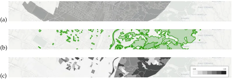
Figure 1 depicts the process of computing the green area coverage indicator. The ge-ometries of census cells in the city are obtained from the Italian statistical office. These constitute theinput set. Next, we query OSM, ourcontextual set, for data describing the surroundings. We take only data about woods, parks, and gardens. These features are ourpoints of interest, conveniently referred to as thePOI set. Both the input and the POI sets are related throughgeometric intersectionto compute the indicator for each census cell. Values for this indicator are used in Figure 1c, where cells with darker colours correspond to greater green area coverage.
(a)
(b)
(c)
© OpenStreetMap contributors (http://www.openstreetmap.org/copyright) © Carto (https://carto.com/attributions)
Figure 1: Computing green area coverage for the city of Turin requires (a) the input set with the city’s census cells and (b) a POI set with green area polygons to produce (c) a map using the coverage ratio as the colouring variable.
Although Figure 1 describes a seemingly straightforward process, we will see in the following sections that there are several challenges in extracting and using crowd-sourced geographical data such as OSM. These challenges arise from the analysis of the contextual dataset and can be classified as follows:
• Discrepancy of taxonomies. This occurs when the alignment between the contex-tual features described in the indicator and the representation of these features in the dataset is not perfect. It may require iterating on query definitions until all needed features are retrieved. Our driving example uses OSM and requires us to get informa-tion about green areas. These are not directly represented in OSM as such. Instead, OSM uses the concepts of parks and gardens. To bridge the gap in this case, we use the Overpass API to retrieve a union of both sets.
• Variations in coverage, specificity, and richness. Data quality may vary from place to place, possibly requiring the use of very different queries depending on the annota-tion style used by the contributor. In OSM, some features are described only by name (e.g., the harbor in Bari uses the key-value pairname=“Bacino della Stazione Marittima") while in other cases features of the same type use more precise descriptions (e.g., the harbor of Sampierdarena also contains the key-value pairharbour=yes).
• Duplicate entities. Crowd-sourced databases, due to their very nature, can contain duplicate annotations about the same entity from different contributors. More of-ten than not, there will be a need to deal with these repetitions before being able to compute the indicator. A specific case in OSM are schools that use the key-value pairamenity=schoolfor individual entrances as well as for the area that represents the school.
• Mixed representations for the same type of feature.The contextual dataset contains more than one way of representing contextual features of the same type, in the same location. Depending on the spatial relation used, this may require that all the features are transformed to use the same representation. In our driving example, we find bus stops being represented both as nodes and as ways in OSM, and substitute those ways with their centroids to provide a uniform representation for the computation function.
the methodology we propose in this paper, however when and how to perform the anal-ysis of the contextual set regarding each one of the above mentioned challenges is part ofMethOSMand will be detailed in the next section (while in Section 5 we perform this analysis for the specific case of our driving example).
4
MethOSM
: a methodology for computing OSM-derived
indicators
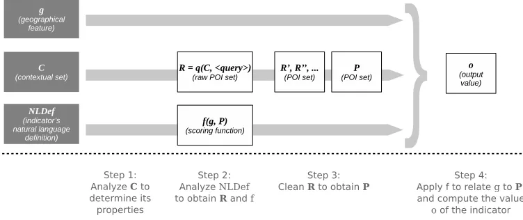
The computation of an indicator is achieved when ascoring functionthat realizes the seman-tics of the indicator is evaluated. TheMethOSMapproach assumes that these semantics are provided as aninformal descriptionwhich guides the analysis to identify certain elements. These elements are then used to define the scoring function and evaluate it. Figure 2 depicts the overall approach. Dark-coloured boxes to the left represent thea priori knowledgefrom which the rest of the elements in the figure are determined. The arrows show three flows of the analysis that allow for the determination of each element from elements to its left. The execution of the methodology is complete when the rightmost elemento, that is, theoutput valueof the scoring function, is determined.
Step 2: Analyze NLDef to obtain R and f Step 1:
Analyze C to determine its properties
Step 3: Clean R to obtain P
Step 4: Apply f to relate g to P, and compute the value
o of the indicator
Figure 2:MethOSMapproach for computing indicators: grey boxes denote input elements required by the approach while white boxes correspond to outputs resulting from the ap-plication of the approach.
The a priori knowledge elements in Figure 2 are defined as follows:
• the geographical featuregfor which the indicator will be computed, • the contextual setCof all features that surroundg, and
• the indicator’s natural language definition (NLDef) that describes the indicator and states howCandgare related.9
9In order for the methodology to be applicable,NLDefneeds to include details about the spatial relations used
The methodology guides the analysis ofNLDef to select, clean, and transform elements inC. This is done in order to define a setPof points of interest containing only the elements ofCthat are involved in the description of the indicator. In order to defineP, it may be necessary to perform a series of refining steps that operate on arawsubset ofC.
This raw subset is represented byR, theraw POI set, and is defined by means of a query functionqthat selects some elements ofC.Ris refined intoR0,R00and so on, performing tasks such as cleaning, deduplicating, and transforming to representations that are required by ascoring functionf to determine the value of the indicator. Functionf is defined from the relation described inNLDef betweengandC.
MethOSM performs this process of finding P and f from the informal description
NLDef in a series of steps that are introduced below.
Step 1: analysis of the contextual set. Before attempting specific tasks related to a partic-ular indicator, it is important to identify potential challenges that can arise from working with the contextual set. The analysis in terms of these challenges will guide decisions taken in steps further down the line for all tasks dealing with the contextual set. A typical set of challenges include:
A Discrepancy of taxonomies between the contextual set and the indicator defini-tion. A geographical indicator describes something about an entity in relation to its surroundings. To gather the input needed from these surroundings, the whole contextual set is queried to retrieve only features that are relevant according to the definition of the indicator. In some cases, there is a trivial translation of what is de-scribed inNLDef into queries to the contextual set. In most cases the alignment is not perfect: taxonomies are different and a non-trivial mapping is needed to reconcile these differences.
B Variations in coverage, specificity, and richness of annotations.Contextual sets of-ten present great variability in annotation quality. Sometimes this variability is seen by comparing one location to another for the same type of feature. Other times the differences are seen across types of features. In both cases, completeness, accuracy, and richness depend heavily on the community of annotators and the methodology employed.
C Duplicate entities. The contextual set may contain duplicates (e.g., due to contrib-utors repeatedly using tags on sub-entities rather than on the main entity—see Sec-tion 3 for a specific example). An analysis of the different cases of duplicaSec-tion must be performed to determine which strategies can be applied (e.g., deduplicate whenever there is an overlap or if features are closer than a certain distance).
D Mixed representations for the same type of feature. Features in the contextual set can be described in many ways (e.g., sometimes as a point that describes roughly where the feature is located and some other times as a polygon describing its exact location and area). Depending on the spatial relation specified in the definition of the indicator, it will be necessary or desirable to reduce all features to the same represen-tation type.
At the end of Step 1 the properties of the contextual set are known and potential chal-lenges are identified.
Step 2: analysis of the indicator’s natural language definition. In this step,NLDef is analyzed to determine two elements:
• A queryq to produce araw POI setR. This queryq will retrieve only the features in the contextual setCthat are points of interest according toNLDef. The process of determiningqis guided by the analysis performed in Step 1. It takes into accountA
andBto bridge any discrepancies and to minimize differences in coverage, specificity, and richness of annotations from location to location. The resulting raw setR is not yet ready to use. It possibly includes duplicates that need to be eliminated and heterogeneous representations that need to be harmonized.
• The scoring functionf that will be applied to produce values for the indicator. This functionf spatially relatesgto points of interest inPand then uses these relations to produce a numerical description according toNLDef.
We define three scoring functions and three spatial relations to illustrate this step. This list is by no means exhaustive and is determined solely by the requirements of the tors presented in Section 3 where we describe our driving example. Other kinds of indica-tors will require different scoring functions and spatial relations not listed here. The scoring functions of our driving example are defined in terms of spatial relations of containment, distance, and area intersection to compute the indicators by usinggandPas input:
• Count nearby.Defined as:
countN earby(g,P, d) ={p|p∈P ∧ distance(g, p)≤d}
(1)
wheredistancedenotes the usual geographical distance and only the POIsp ∈ P, contained within a circle defined using the distancedfromgare selected. The count is the number of elements of the resulting set.
• Closest distance.Defined as:
closestDistance(g,P) = min
∀p∈Pdistance(g, p) (2)
whereclosestDistanceis the minimum distance fromgto all the POIsp∈P. • Shared to total ratio.Defined as:
ratioSharedT otal(g,P) =area(shared(g,P))
area(g) (3)
whereareais defined in the usual way as the extent of a geographical surface. The sharedfunction is defined as:
shared(g,P) =
n
G
j=1
gupj pj∈P, n=
P
(4)
At the end of Step 2 we obtain the raw POI setRand the definition off, the scoring function to compute the indicator forg.
Step 3: cleaning of the POI set. In order to apply the scoring functionf, we need to transform the raw POI setRinto the clean versionP. The analysis done in Step 1 should be used as guidance to achieve this.
In the case of our driving example, as a result of the analysis ofRin light of challengeC, we identify different cases of duplicate entities inRand the consequent need for dedupli-cation in order to transformRinto the clean versionP. We present the two deduplication strategies applied in our driving example:
• Deduplication by intersection. The elimination is done by detecting intersection areas between points of interest, preferring the more descriptive version over the less descriptive one.
dedupByIntersection(R) ={r|r, q∈R ∧ ruq=∅} ∪ {r|r, q∈R ∧ r6=q ∧ ruq6=∅ ∧ isP olygon(r)} ∪ {q|r, q∈R ∧ r6=q ∧ ruq6=∅ ∧ ¬isP olygon(r)}
(5)
where∪is the set union andisP olygonistrueonly when the element is a polygon. In this way, allr∈Rare selected if there is no intersection. If there is an intersection, the polygon representation is preferred.
• Deduplication by proximity. The elimination is done by treating points of interest that are closer than a threshold as being the same entity.
dedupByP roximity(R, d) ={r|r, q∈R ∧ distance(r, q)> d} ∪ {r|r, q∈R ∧ r=6 q ∧ distance(r, q)≤d ∧ isP olygon(r)} ∪ {q|r, q∈R ∧ r=6 q ∧ distance(r, q)≤d ∧ ¬isP olygon(r)}
(6)
whered is the threshold distance to consider that there is proximity between two elements.
In this way, allr∈Rare selected if there is no proximity withq. If there is proximity, the polygon representation is preferred.
FromD we identify different ways in which points of interest are represented in R. Next, we assess the impact that these different representations have on the requirements of the scoring functionf. There is a need to homogenize if not all the different representations can be used as input forf.
In other cases, there are features that simply lack the information necessary to be used as input. f requires a more complex representation and thus the only possible strategy is to discard those features.
The implementation of the strategies to tackle challengesCandDwas achieved using PostgreSQL queries with functions provided by the PostGIS extension, although several current GIS toolkits should be up to the task.
At the end of Step 3 we obtain a clean POI setPthat can be used to evaluatef.
Step 4: computation of the indicator. Once the scoring functionf and the POI setPare known, we can compute the value of the indicator forg.
The process can be optimized if we establish ahorizonfor the contextual setC, centred ong. This horizon establishes awindowfor queryingC, thus restricting the indicator to only describing phenomena inside the window defined by the horizon.
The horizon is selected in order to include all relevant features, assuming that there is a maximum distance beyond which there is no useful information for the computation. We propose thebounding boxapproach to define the horizon: the centroid ofgis taken and the box is defined by transposing coordinates by a fixed distance in meters in all four cardinal points. We selected the bounding box approach due to its lightweight nature, although other approaches such as defining the horizon as a circumference of a certain radius from the centroid ofgwill produce the same results.
At the end of Step 4 we obtain the outputo, that is, the value of the indicator forg.
Although we discussed scoring functions in Step 2 and cleaning strategies in Step 3, these are specific results of the application of the methodology in our driving example and for the case of OSM. Other datasets will present different situations and require different strategies that could require dataset-specific domain knowledge on the part of the data scientist. The goal of the methodology is to ease the task of defining the scoring function and of obtaining a suitable contextual set by analyzing the problem in the proposed four steps.
5
Exemplifying
MethOSM
for computing indicators
In Section 4 we presentedMethOSMto compute indicators starting from an informal defi-nitionNLDef of the indicator, a geographical featuregon which to compute the indicator and a contextual setCthat describes the surroundings ofg. In this section we show how we apply the methodology to our driving example, in order to compute each one of its indicators. The geographical featuregis the same in all cases: a polygon representing a census cell in the city of Turin. In the same way, OSM is the contextual setCshared among all indicators. We will query OSM to build our POI set P. To this end, we will define queries using Overpass QL10.
To applyMethOSM, first we describe Step 1 (the analysis of the contextual set) as this step is shared among all three indicators in our running example. Next, we perform the steps particular to each indicator in Subsections 5.1, 5.2 and 5.3, respectively.
Step 1: analysis of the contextual set. We analyze the challenges described in Section 4 in light of our driving example:
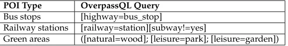
A Discrepancy of taxonomies between the contextual set and the indicator definition. We find that in some cases there is a direct correspondence to a class of features in OSM (e.g., bus stops in OSM are represented with thehighway=bus_stopkey-value pair). In other cases there can be a partial correspondence which needs a more com-plex query. To query for railway stations we have to specifically filter out entrances to the subway network using [railway=station][subway!=yes]. Another example of partial correspondence occurs in the case of green areas: we have to issue a com-plex query that retrieves woods, parks, and gardens, represented as([natural=wood]; [leisure=park]; [leisure=garden]). This analysis is summarized in Table 1.
POI Type OverpassQL Query
Bus stops [highway=bus_stop]
Railway stations [railway=station][subway!=yes]
Green areas ([natural=wood]; [leisure=park]; [leisure=garden])
Table 1: Mapping bus stops, railway stations, and green areas to Overpass QL queries.
B Variations in coverage, specificity, and richness of annotations. In the particular case of OSM, coverage can vary from city to city depending on region and size: bigger cities tend to have higher coverage in general while cities in the North of Italy present higher coverage than cities in the South. When analyzing specificity and richness for different types of features, we see that annotation provenance plays a decisive role. Official agencies have varied policies and spend resources differently; Italian municipal authorities do a good job annotating bus stops while annotation of harbor facilities is at best spotty.
Volunteer efforts often bridge the gap but they can be less rigorous. We found dif-ferent approaches for annotating harbors (e.g., more specificharbour=yesversus less precisename=“Bacino della Stazione Marittima”), often requiring a search for specific harbor names to get their locations instead of resorting to looking for the more suit-ablekey-valuecombination.
Fortunately, for our driving example, which spans a relatively small area (i.e., the city of Turin), the quality of annotations for all types of points of interest is sufficiently ad-equate. In other cases a possible solution would require location-dependent queries. That is, there would be the need to specify custom queries attached to specific loca-tions to supersede generic ones.
C Duplicate entities. OSM is kept up-to-date by the combined effort of countless an-notators. By their very nature, such crowd-sourced efforts are very decentralized and there is no easy way to avoid errors in the annotation task.
In some cases, the same entity is annotated several times by independent annotators. Consequently, some processing must be done to discard duplicates. In our driving ex-ample, some railway stations are mapped more than once, first as an area and again as a node, without a relation that links them. These cases can be systematically spotted as the distance between duplicates is zero or near-zero.
We deal with this situation when we count nearby bus stops for census cells within the city of Turin. In OSM, bus stops are often described using single points, although in some cases annotators have instead provided polygons that map the waiting area of these bus stops. These differences in dimensionality, when present, need to be taken into account before applying the spatial relation needed to compute an indica-tor.
A similar situation occurs also for railway stations and green areas. Some instances are thoroughly represented as polygons that give information about the area covered by the feature while other instances only give a general location as a point.
5.1
Number of nearby bus stops indicator
Step 2: analysis of the indicator’s natural language definition. This indicator can be informally defined as:
NLDef: the number of nearby bus stops to each of the census cells in the city, where
a bus stop is considered to be nearby if the distance between it and the cell is at most 500 meters.
An analysis ofNLDef determines the following:
• The raw POI setRis obtained by queryingC(i.e., OSM, our contextual set) for bus stops, according to Table 1:
R=q(C) =overpass(C,“highway=bus_stop”)
whereoverpassrepresents the query function in OverpassQL,Ris thepossibly raw
set of features in the contextual setCthat represent bus stops.
• The scoring functionf that relatesgwith the POI setP:
f =countN earby(g,P,500) (7)
wherecountN earbyis as defined in (1).
Step 3: cleaning of the POI set. InCwe determined thatRcontains duplicate bus stops. To come up with a sensible cleaning strategy, we identified different cases of duplication:
• The bus stop being represented more than once with increasing degrees of complexity (i.e., as a point representing the general location of the bus stop, and as a polygon describing the exact waiting area for passengers);
• The feature being accidentally represented more than once due to contributor errors.
In the first case, the issue can be solved by applyingdedupByIntersectionas defined in (5), discarding all points inside polygons:
R0 =dedupByIntersection(R)
For the second case,dedupByProximityas defined in (6) will be enough to discard un-wanted repetitions:
R00=dedupByP roximity(R0,3)
where 3 meters is the threshold distance we selected to assume that two features are the same andR00is the set resulting from the application of the strategy.
FromDwe know that our set of bus stopsR00contains heterogeneous representations. Given the fact that the bus stops represented as polygons span a reduced area, we can substitute these polygons by their centroids with a negligible impact on accuracy:
P=reduceByCentroid(R00)
wherePis the clean, homogeneous set of points representing bus stops.
Step 4: computation of the indicator. Once Pis determined, we are ready to find the outputoforgby applyingf as defined in (7):
o=countN earby(g,P,500)
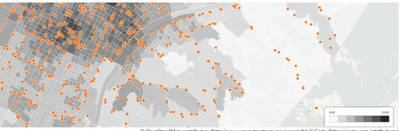
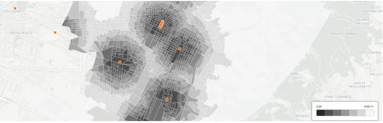
Figure 3 shows a choropleth map of Turin census cells using the indicator as the colour-ing variable.
© OpenStreetMap contributors (http://www.openstreetmap.org/copyright) © Carto (https://carto.com/attributions)
Figure 3: Census cells by number of nearby(d ≤500m)bus stops. Features representing bus stops are overlaid to provide reference.
5.2
Distance to the closest railway station indicator
Step 2: analysis of the indicator’s natural language definition. This indicator can be informally defined as:
NLDef: the distance from the centroid of each census cell in the city to the closest
railway station, where the distance is measured in meters.
• The raw POI set R is obtained by querying C for railway stations, according to Table 1:
R=q(C) =overpass(C,“[railway=station][subway! =yes]”)
where R is the possibly raw set of features in the contextual set C that represent railway stations.
• The scoring functionf that relatesgwith the POI setP:
f =closestDistance(g,P) (8)
whereclosestDistanceis as defined in (2).
Step 3: cleaning of the POI set. InCwe determined thatRcontains more than one rep-resentation referring to the same railway station.
Unlike the case in Section 5.1, the impact of duplicates is negligible for finding the dis-tance to the closest railway station in the city of Turin. This is due to (8) selecting the closest distance regardless of the number of times the same feature is represented.
FromDwe know that our setRof railway stations contains heterogeneous representa-tions. After inspection, we determined that the centroids of railway stations are closer to where railway users need to reach to use the railway service than points in the perimeter of polygon representations. Through homogenization, we obtain more useful representations of each railway station:
P=reduceByCentroid(R)
wherePis the clean set of points representing railway stations andreduceByCentroidis a function that finds the geometric centroid for each element inRto buildP.
Step 4: computation of the indicator. OncePis determined, we are ready to find the outputoforgby applyingf as defined in (8):
o=closestDistance(g,P)
Figure 4 shows a choropleth map of Turin census cells using the indicator as the colour-ing variable.
5.3
Green area coverage indicator
Step 2: analysis of the indicator’s natural language definition. This indicator can be informally defined as:
NLDef: the ratio of green area (parks, woods, gardens) to total census cell area.
An analysis ofNLDef determines the following:
• The raw POI set R is obtained by querying C for features that represent parks, woods and gardens. According to Table 1:
© OpenStreetMap contributors (http://www.openstreetmap.org/copyright) © Carto (https://carto.com/attributions)
Figure 4: Census cells by distance to the closest railway station. Railway station features are overlaid to provide reference.
whereRis thepossibly rawset of features in the contextual setCthat represent green areas.
• The scoring functionfthat relatesgwith the POI setP:
f =ratioSharedT otal(g,P) (9)
whereratioSharedT otalis as defined in (3).
Step 3: cleaning of the POI set. InCwe determined thatRcontains more than one rep-resentation referring to the same green area. Two cases were found:
• parks represented both as a polygon and as a point and • parks annotated twice or more as polygons.
The first case is handled taking into account our analysis inD; we cannot work with point representations to compute the green area coverage. We need to discard point representa-tions:
R0=discardP oints(R) whereR0is a set that contains only polygons.
The second case will be handled in the Step 4, since ratioSharedTotal makes use of
shared, as seen in (3). Note thatsharedusest, seen in (4), to compute the union between all
green area polygons. This has a convenient side-effect: repeated green areas that overlap are taken into account just once. Consequently, R0 is ready to be used as input for the scoring function:
P=R0
Step 4: computation of the indicator. Once Pis determined, we are ready to find the outputoforgby applyingf as defined in (9):
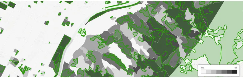
Figure 5 shows a choropleth map of Turin census cells using the indicator as the colouring variable.
© OpenStreetMap contributors (http://www.openstreetmap.org/copyright) © Carto (https://carto.com/attributions)
Figure 5: Census cells by ratio green area to total cell area. Green area polygons are overlaid to provide reference.
6
Discussions and validation of
MethOSM
for computing a
complex indicator
In order to validate the proposed methodology in a larger setting, we used it for computing a complex indicator. The complex indicator describes a socio-economic phenomena—that of understanding how the value of real estate properties changes over time.
The indicators introduced in the previous sections were used to build the complex indi-cator used in an Automated Valuation Model (AVM) that estimates the value of real estate properties. In a nutshell, zones with higher scores for mass transportation and greater green area coverage presume to contain more valuable properties. This composite indi-cator was developed for Cerved, a credit scoring company in Italy11, as part of Cerved’s Cadastral Report Service (CCRS)12 aiming to objectively estimate the value of real estate properties in Italy by using different types of datasets (open data / OSM, proprietary data, and third-party data). Valuation of real estate properties is a challenging task and requires accumulation and processing of different types of information about properties, including contextual information about their locations, such as economic and social trends, environ-mental conditions, proximity to the historical center, and concentration of managers’ and shareholders’ households [34], to name a few. This task is typically performed by expert evaluators who visually inspect the property. As such it is a long, expensive, and error-prone process which is mostly qualitative and based on implicit knowledge.
The objective of CCRS was to automate this task by building an AVM integrating com-posite indicators that could estimate values for real estate properties. Moreover, it was crucial for the service to be able to compute the indicator for the entire Italian territory.
11https://www.cerved.com
12More details about the CCRS business case can be found at https://blog.prodatamarket.eu/2015/06/
OSM was chosen as a source of contextual territorial information. Starting from the exact location of a property, the property is mapped to the corresponding census cell and the related territorial scores. For each census cell, different indicators were computed based on the different sources available, in a hierarchical manner, following theMethOSM method-ology, to arrive to an integrated final score used by the estimation algorithm (i.e., the real estate integrated score). These indicators computed per census cell were:
• Social discomfort index (IDS): based on social and demographic variables from the IS-TAT national census of 2011.
• Real estate discomfort index (IDE): based on the state of conservation of properties from the ISTAT national census of 2011.
• Social demographic score: based on IDS and IDE.
• Manager and Shareholder Concentration (MSHC) score: based on Cerved official and proprietary data about the presence of managers and shareholders in the area. • People score: based on the integration of MSHC and the Social demographic score. • Heavy Industrial Concentration (HIC) score: based on Cerved official and proprietary
data about the concentration of industries in certain NACE13categories.
• Territory score: based on HIC and other variables about territorial features. Among these territorial features, the following OSM-derived indicators were used: number of nearby bus stops, distance to the nearest railway station, green area coverage, to-tal length of pedestrian paths in the vicinity, number of sites of historical relevance, number of nearby hotels and hotel-related features, ratio of land for industrial use to total cell area, and distance to the nearest coast (where applicable).
• Real estate integrated score: based on the integration of the People and Territory scores.
For the Territory score, in addition to the three indicators computed in Section 5,
MethOSM was used to guide the analysis for the five other indicators mentioned above. In the following list we discuss some of the peculiarities of the application ofMethOSM, compared to the indicators discussed in Section 5:
• Total length of pedestrian paths in the vicinity.After a preliminary analysis, it was determined that the best alignment with the intended definition of pedestrian path was produced by the query that retrieved features tagged with at least one of high-way=pedestrian, highway=footway, highway=ciclewayand highway=steps. To clean the raw POI setR, we eliminated all features that were single points or polygons, leav-ing only lines. The scorleav-ing function selected all paths within a radius of 1000 meters from the centroid of the census cell.
• Number of sites of historical relevance. After a preliminary analysis, it was de-termined that the relevant tags weretourism=museum, historic=ruins, historic=yes, his-toric=castle and historic=building. The annotation on the area representation was pre-ferred for overlapping annotations. The reasoning for the scoring function was simi-lar to the case described in Section 5.1 for “number of nearby stops.”
• Number of nearby hotels and hotel-related features. In this case, we
de-termined that the relevant OSM tags were tourism=hotel, tourism=hostel and
tourism=guest_house. The deduplication strategy chosen was the same as in the previ-ous case.
13EC NACE: http://ec.europa.eu/eurostat/statistics-explained/index.php/Glossary:
• Ratio of land for industrial use to total cell area. Here the OSM taxonomy is well aligned with the intended meaning of industrial land use. Polygon representations tagged withlanduse=industrialwere retrieved and used in a scoring function similar to the case described in Section 5.3 for “green area coverage.”
• Distance to the nearest coast. In this case there is a good alignment between the OSMnatural=coastline and the concept of coast required by the indicator. The POI set obtained by issuing the query contained only open paths that represented lines. Consequently, no further transformations were required. The scoring function was analogous to the case described in Section 5.2 for “distance to the closest railway station.”
MethOSMwas successfully employed to compute the OSM-derived indicators for the whole of Italy: more than 400,000 census cells in 7,978 municipalities and 20 regions, in-cluding rural areas, villages, towns, and cities in the following configurations: coastal, inland, and mountain. The reason for computing the OSM-derived indicators in differ-ent configurations and weighting them differdiffer-ently in the final composite indicator was to take into account variations in availability and quality of the data in various areas. In or-der to measure the quality of the resulting indicator, one has to compare it to a “golden standard.” In our case of the indicator estimating the value of real estate properties the only way to check how good it is was to compare it to a corresponding indicator calcu-lated based on historical data on real estate transactions (data available from the Italian government, though not open data), i.e., the “golden standard.” The computed indicator closely followed the “golden standard,” meaning that the employed data and method were sound for this particular problem. This required the computation of the OSM-derived in-dicators in different configurations as mentioned above, and adjusting their weights in the final composite indicator till a close enough match to the “golden standard” was obtained.
MethOSMplayed a key role in guiding the process for harmonizing the complex process of dealing with OSM data for computing the various indicators, making the overall task of computing OSM-derived indicators efficient and effective. Indicators from this business case were made available as Linked Data in [40] through the DataGraft platform14[36, 37]. The applicability of this complex indicator to another country depends on several fac-tors. First, for computing the scores that use proprietary data (e.g., data about presence of managers and shareholders in a given area), similar data would need to be obtained for that country. Typically this is commercial data and not open. Further, the structure of this proprietary data would need to be similar to the one used for computing the indicator for Italy, likely requiring some transformations. Second, for the OSM-derived indicators several aspects would need to be take into consideration. For example, cultural differences may result in concepts such asnearbybeing defined differently. Additionally, the alignment work for OSM to match the intended meaning contained in the natural language definition of the indicator may produce different results depending on the annotation methodologies used from location to location. Consequently, also the deduplication strategies may need adjustments to reflect this fact.
7
Conclusions and outlook
With the availability of increasing volumes of data, new opportunities are opened for the development of various composite indicators to define and analyze complex social, eco-nomic, political, or environmental phenomena. The emergence of open data is especially relevant as it has enabled individuals and businesses the access to affordable data on top of which interesting indicators can be computed. An example of such an open dataset is OSM which has been used as a baseline dataset for computing indicators, for example, in areas where official data did not exist, or simply because OSM data is freely available and can be easily accessed. Previous work on computing indicators derived from OSM has shown a number of challenges in extracting and using data for computing indicators, with ad-hoc, often overlapping solutions being developed to address the challenges. In this context, this paper proposed (and formalized)MethOSM—a systematic methodology for computing indicators derived from OSM data, with the aim of supporting individuals with a clear set of steps and help them identify a set of issues that need to be addressed for an effective and efficient computation. To that end, we exemplified the successful use of the proposed methodology on a number of indicators that use OSM as the contextual source, and validated the methodology for computing a complex indicator in a real business case for estimating the value of real estate properties using OSM data.
We consider the methodology proposed in this paper generic in the sense that it can be used with other contextual datasets. To this end, we plan to investigate the use ofMethOSM
with contextual datasets other than OSM such as the Italian Car Fleet Database15to describe fleet configurations by municipality and region and the Atoka Company Database16 to model phenomena related to economic activity throughout Italy. The study of these contex-tual datasets will add to the list of challenges introduced in Step 1 in the current version of
MethOSM. With a more exhaustive list, it should be possible to introduce a more systematic approach to the analysis of the contextual dataset. The study of other well-known reference datasets should result in the identification of a set of cleaning and deduplication strategies and a description of the conditions in which each strategy can be applied. Additionally, an analysis of the different representations and spatial units in use could result in exten-sions toMethOSMthat deal with these differences in an automatic or semi-automatic way. Moreover, the application ofMethOSMto compute new types of indicators will most likely add to the scoring function types now present in Step 2. The next iteration ofMethOSM
will introducefeature selectorsandfeature evaluatorsto further describe the process of trans-forming natural language definitions into scoring functions. Future work can include the use of OSM to compute indicators based on more complex distance algorithms such as walking distance, driving distance, and commuting distance. Comparison ofMethOSM re-sults against a dataset of commuting times in metropolitan areas could open an interesting avenue for performance evaluation. Another avenue for potential future work could be related to biases (e.g., socio-political) introduced in OSM data during its production and how such biases could be taken into account inMethOSM. On one hand, we foresee cer-tain improvements of the data extraction procedures. As demonstrated in [20] positional accuracy of OSM data increases with the amount of contributors who worked on a given spatial unit of OSM. It is worth exploring whether this and possibly other intrinsic data properties could be used to improve data extraction and data cleansing procedures of our
methodology. On the other hand, fundamental studies on the imprint of social inequali-ties and digital divide on VGI question consistency and utility of VGI as a category [8, 9]. It is important to incorporate data about demographics of the OSM contributors into our extraction procedures, so that the users of the methodology can decide whether and how to utilize such data.
Acknowledgments
This work has been partly funded by the European Commission through the projects proDataMarket (Grant number: 644497), euBusinessGraph (Grant number: 732003), EW-Shopp (Grant number: 732590), and TheyBuyForYou (Grant number: 780247).
References
[1] AGNOLETTI, M., CONTI, L., FREZZA, L.,ANDSANTORO, A. Territorial analysis of the agricultural terraced landscapes of Tuscany (Italy): Preliminary results. Sustainability 7, 4 (2015), 4564–4581. doi:10.3390/su7044564.
[2] AMELUNXEN, C. On the suitability of volunteered geographic information for the purpose of geocoding.Proceedings of the geoinformatics forum salzburg(2010).
[3] ARSANJANI, J. J., BARRON, C., BAKILLAH, M., AND HELBICH, M. Assessing the quality of OpenStreetMap contributors together with their contributions. In16th AG-ILE international conference on geographic information science(Leuven, Belgium, 2013), pp. 14–17.
[4] ARSANJANI, J. J., MOONEY, P., ZIPF, A.,ANDSCHAUSS, A. Quality assessment of the contributed land use information from OpenStreetMap versus authoritative datasets. InOpenStreetMap in GIScience. Springer, 2015, pp. 37–58. doi:10.1007/978-3-319-14280-7_3.
[5] ARSANJANI, J. J., ZIPF, A., MOONEY, P., AND HELBICH, M. OpenStreetMap in GI-Science: Experiences, Research, and Applications. Springer Publishing Company, Incor-porated, 2015. doi:10.1007/978-3-319-14280-7.
[6] BAKILLAH, M., LIANG, S., MOBASHERI, A., ARSANJANI, J. J., AND ZIPF,
A. Fine-resolution population mapping using OpenStreetMap points-of-interest.
International Journal of Geographical Information Science 28, 9 (2014), 1940–1963. doi:10.1080/13658816.2014.909045.
[7] BECCARI, B. A comparative analysis of disaster risk, vulnerability and resilience composite indicators. PLOS Currents Disasters (March 2016). doi:10.1371/currents.dis.453df025e34b682e9737f95070f9b970.
[9] BITTNER, C. OpenStreetMap in Israel and Palestine—‘game changer’ or re-producer of contested cartographies? Political Geography 57 (2017), 34 – 48. doi:doi:10.1016/j.polgeo.2016.11.010.
[10] BOLSTAD, P. GIS Fundamentals: A First Text on Geographic Information Systems. Eider Press, 2005.
[11] CAMBOIM, S. P., BRAVO, J. V. M., AND SLUTER, C. R. An investigation into
the completeness of, and the updates to, OpenStreetMap data in a heterogeneous area in Brazil. ISPRS International Journal of Geo-Information 4, 3 (2015), 1366. doi:doi:10.3390/ijgi4031366.
[12] DEVILLERS, R., STEIN, A., BÉDARD, Y., CHRISMAN, N., FISHER, P., AND SHI, W. Thirty years of research on spatial data quality: achievements, failures, and opportu-nities.Transactions in GIS 14, 4 (2010), 387–400. doi:10.1111/j.1467-9671.2010.01212.x.
[13] DORN, H., TÖRNROS, T.,ANDZIPF, A. Quality evaluation of VGI using authoritative
data—a comparison with land use data in southern Germany. ISPRS International Journal of Geo-Information 4, 3 (2015), 1657–1671. doi:10.3390/ijgi4031657.
[14] ELWOOD, S., GOODCHILD, M. F., AND SUI, D. Z. Researching volunteered geographic information: Spatial data, geographic research, and new social prac-tice. Annals of the Association of American Geographers 102, 3 (2012), 571–590. doi:10.1080/00045608.2011.595657.
[15] ESTIMA, J., ANDPAINHO, M. Exploratory analysis of OpenStreetMap for land use
classification. In Proceedings of the Second ACM SIGSPATIAL International Workshop on Crowdsourced and Volunteered Geographic Information(New York, NY, USA, 2013), GEOCROWD ’13, ACM, pp. 39–46. doi:10.1145/2534732.2534734.
[16] FUENTES-VALLEJO, M., HIGUERA-MENDIETA, D. R., GARCÍA-BETANCOURT, T., ALCALÁ-ESPINOSA, L. A. C., GARCÍA-SÁNCHEZ, D., MUNÉVAR-CAGIGAS, D. A., BROCHERO, H. L., GONZÁLEZ-URIBE, C., AND QUINTERO, J. Territorial analy-sis of aedes aegypti distribution in two Colombian cities: a chorematic and ecosys-tem approach. Cadernos de Saúde Pública 31(03 2015), 517 – 530. doi:10.1590/0102-311X00057214.
[17] GIL, J. Building a multimodal urban network model using OpenStreetMap data for the analysis of sustainable accessibility. InOpenStreetMap in GIScience. Springer, 2015, pp. 229–251. doi:10.1007/978-3-319-14280-7_12.
[18] GOODCHILD, M. F. Citizens as sensors: the world of volunteered geography. GeoJour-nal 69, 4 (Aug 2007), 211–221. doi:10.1007/s10708-007-9111-y.
[19] HAKLAY, M. How good is volunteered geographical information? A comparative
study of OpenStreetMap and ordnance survey datasets. Environment and Planning B: Planning and Design 37, 4 (2010), 682–703. doi:10.1068/b35097.
[21] HARDEMAN, S., VAN ROY, V., VERTESY, D., AND SAISANA, M. An analysis of na-tional research systems (I): A composite indicator for scientific and technological re-search excellence. doi:10.2788/95887.
[22] JAH ¯¯ ANA, S. Human development report 2016: human development for everyone.
doi:10.18356/6d252f18-en.
[23] KAMAL, S. H. M., RAFIEY, H., SAJJADI, H., RAHGOZAR, M., ABBASIAN, E., AND
SANI, M. S. Territorial analysis of social welfare in Iran. Journal of International and Comparative Social Policy 31, 3 (2015), 271–282. doi:10.1080/21699763.2015.1095580.
[24] LI, Q., FAN, H., LUAN, X., YANG, B., AND LIU, L. Polygon-based ap-proach for extracting multilane roads from OpenStreetMap urban road networks.
International Journal of Geographical Information Science 28, 11 (2014), 2200–2219. doi:doi:10.1080/13658816.2014.915401.
[25] LUDWIG, I., VOSS, A., ANDKRAUSE-TRAUDES, M. A comparison of the street net-works of Navteq and OSM in Germany. InAdvancing geoinformation science for a chang-ing world. Springer, 2011, pp. 65–84. doi:10.1007/978-3-642-19789-5_4.
[26] MAZZOCCHI, C., SALI, G.,ANDCORSI, S. Land use conversion in metropolitan
ar-eas and the permanence of agriculture: Sensitivity index of agricultural land (SIAL), a tool for territorial analysis. Land Use Policy 35, Supplement C (2013), 155 – 162. doi:10.1016/j.landusepol.2013.05.019.
[27] MOBASHERI, A., SUN, Y., LOOS, L., AND ALI, A. L. Are crowdsourced datasets suitable for specialized routing services? Case study of OpenStreetMap for routing of people with limited mobility.Sustainability 9, 6 (2017), 997. doi:10.3390/su9060997.
[28] MOCNIK, F.-B., MOBASHERI, A., GRIESBAUM, L., ECKLE, M., JACOBS, C., AND
KLONNER, C. A grounding-based ontology of data quality measures.Journal of Spatial Information Science 2018, 16 (2018), 1–25. doi:10.5311/JOSIS.2018.16.360.
[29] MOCNIK, F.-B., MOBASHERI, A.,ANDZIPF, A. Open source data mining infrastruc-ture for exploring and analysing OpenStreetMap. Open Geospatial Data, Software and Standards 3, 1 (2018), 7. doi:10.1186/s40965-018-0047-6.
[30] MOONEY, P., ANDCORCORAN, P. Characteristics of heavily edited objects in Open-StreetMap.Future Internet 4, 1 (2012), 285–305. doi:10.3390/fi4010285.
[31] MOONEY, P., AND CORCORAN, P. Analysis of interaction and co-editing patterns amongst OpenStreetMap contributors. Transactions in GIS 18, 5 (2014), 633–659. doi:10.1111/tgis.12051.
[32] NEIS, P., ANDZIELSTRA, D. Recent developments and future trends in volunteered geographic information research: The case of OpenStreetMap. Future Internet 6, 1 (2014), 76–106. doi:10.3390/fi6010076.
[34] POZZATI, S., SANVITO, D., CASTELLI, C., ANDROMAN, D. Understanding territo-rial distribution of properties of managers and shareholders: a data-driven approach.
Territorio Italia, 2 (2016), 27–40. doi:10.14609/Ti_2_16_2e.
[35] ROICK, O., HAGENAUER, J.,ANDZIPF, A. OSMatrix–grid–based analysis and visual-ization of OpenStreetMap. InProceedings of the 1st European State of the Map Conference (SOTM-EU)(Vienna, Austria, 2011).
[36] ROMAN, D., DIMITROV, M., NIKOLOV, N., PUTLIER, A., SUKHOBOK, D., ELVESÆTER, B., BERRE, A., YE, X., SIMOV, A., AND PETKOV, Y. Datagraft: Sim-plifying open data publishing. InEuropean Semantic Web Conference(2016), Springer, pp. 101–106. doi:10.1007/978-3-319-47602-5_21.
[37] ROMAN, D., NIKOLOV, N., PUTLIER, A., SUKHOBOK, D., ELVESÆTER, B., BERRE,
A., YE, X., DIMITROV, M., SIMOV, A., ZAREV, M., MOYNIHAN, R., ROBERTS, B.,
BERLOCHER, I., KIM, S., LEE, T., SMITH, A., ANDHEATH, T. DataGraft: One-stop-shop for open data management. Semantic Web 9, 4 (2018), 393–411. doi:10.3233/SW-170263.
[38] SCHLESINGER, J. Using crowd-sourced data to quantify the complex urban fabric— OpenStreetMap and the urban–rural index. InOpenStreetMap in GIScience. Springer, 2015, pp. 295–315. doi:10.1007/978-3-319-14280-7_15.
[39] SENARATNE, H., MOBASHERI, A., ALI, A. L., CAPINERI, C., AND HAKLAY, M. A review of volunteered geographic information quality assessment meth-ods. International Journal of Geographical Information Science 31, 1 (2017), 139–167. doi:10.1080/13658816.2016.1189556.
[40] SUKHOBOK, D., DJORDJEVIC, D., SANVITO, D., PANIAGUA, J.,ANDROMAN, D. Pub-lishing socio-economic territory indices as linked data and their visualization for real estate valuation. InProceedings of the ISWC 2017 Posters & Demonstrations and Industry Tracks co-located with 16th International Semantic Web Conference (ISWC 2017), Vienna, Austria, October 23rd - to - 25th, 2017.(2017).
[41] UUEMAA, E., ANTROP, M., ROOSAARE, J., MARJA, R.,ANDMANDER, Ü. Landscape metrics and indices: an overview of their use in landscape research. Living reviews in landscape research 3, 1 (2009), 1–28. doi:10.12942/lrlr-2009-1.
[42] VAZ, E., AND JOKAR ARSANJANI, J. Crowdsourced mapping of land use in urban dense environments: An assessment of Toronto.The Canadian Geographer / Le Géographe canadien 59, 2 (2015), 246–255. doi:10.1111/cag.12170.
[43] YANG, L. An inventory of composite measures of human progress. Occasional Paper on Methodology(2014).
[44] ZARZOSAESPINA, P., AND SOMARRIBA ARECHAVALA, N. An assessment of social