Statistical Methods For Censored And Missing Data In Survival And Longitudinal Analysis

(1)

University of Pennsylvania

ScholarlyCommons

Publicly Accessible Penn Dissertations

2019

Statistical Methods For Censored And Missing Data In Survival

And Longitudinal Analysis

Leah Helene Suttner

University of Pennsylvania, [email protected]

Follow this and additional works at: https://repository.upenn.edu/edissertations

Part of the Biostatistics Commons

Recommended Citation

Suttner, Leah Helene, "Statistical Methods For Censored And Missing Data In Survival And Longitudinal Analysis" (2019). Publicly Accessible Penn Dissertations. 3520.

(2)

Statistical Methods For Censored And Missing Data In Survival And Longitudinal

Analysis

Abstract

Missing or incomplete data is a nearly ubiquitous problem in biomedical research studies. If the incomplete data are not appropriately addressed, it can lead to biased, inefficient estimation that can impact the conclusions of the study. Many methods for dealing with missing or incomplete data rely on parametric assumptions that can be difficult or impossible to verify. Here we propose semiparametric and nonparametric methods to deal with data in longitudinal studies that are missing or incomplete by design of the study. We apply these methods to data from Parkinson's disease dementia studies. First, we propose a quantitative procedure for designing appropriate follow-up schedules in time-to-event studies to address the problem of interval-censored data at the study design stage. We propose a method for generating proportional hazards data with an unadjusted survival similar to that of historical data. Using this data generation process we conduct simulations to evaluate the bias in estimating hazard ratios using Cox regression models under various follow-up schedules to guide the selection of follow-up frequency. Second, we propose a nonparametric method for longitudinal data in which a covariate is only measured for a subset of study subjects, but an informative auxiliary variable is available for everyone. We use empirical and kernel density estimates to obtain nonparametric density estimates of the

conditional distribution of the missing data given the observed. We derive the asymptotic distribution of the estimator for time-varying missing covariates as well as discrete or continuous auxiliary variables and show that it is consistent and asymptotically normally distributed. Through simulations we show that our estimator has good finite sample properties and is more efficient than the complete case estimator. Finally, we provide an R package to implement the method.

Degree Type

Dissertation

Degree Name

Doctor of Philosophy (PhD)

Graduate Group

Epidemiology & Biostatistics

First Advisor

Sharon X. Xie

(3)

STATISTICAL METHODS FOR CENSORED AND MISSING DATA IN SURVIVAL AND LONGITUDINAL ANALYSIS

Leah H. Suttner A DISSERTATION

in

Epidemiology and Biostatistics

Presented to the Faculties of the University of Pennsylvania in

Partial Fulfillment of the Requirements for the Degree of Doctor of Philosophy

2019

Supervisor of Dissertation

Sharon X. Xie, Professor of Biostatistics

Graduate Group Chairperson

Nandita Mitra, Professor of Biostatistics

Dissertation Committee

(4)

c

Leah H. Suttner

This work is licensed under the Creative Commons Attribution NonCommercial-ShareAlike 3.0 License

To view a copy of this license, visit

(5)

ACKNOWLEDGEMENT

First and foremost, I would like to thank my dissertation advisor Dr. Sharon X. Xie. Your knowledge and guidance were invaluable throughout this work. Thank you for your patience and support in teaching me how to be a better statistician and conduct research. Thank you to my committee members, Dr. Sarah J. Ratcliffe, Dr. Susan S. Ellenberg, and Dr. Daniel Weintraub for sharing your time and expertise with me. I would also like to thank Dr. Russell T. Shinohara for his support in my first year of graduate school. Thank you for taking the time to teach me and answer my questions and for making me feel welcome in your lab when I was new.

I also have to thank all of the amazing gradute students, both past and present, that I have met here at Penn. You are an inspiration and I’ve truely valued your freindship. A special shout out to the Pooper Troopers for your support and always helping my to keep pedaling through.

(6)

ABSTRACT

Leah H. Suttner

Sharon X. Xie

(7)

LIST OF TABLES

TABLE 2.1 : HR estimation bias from right-endpoint imputation in univariate and multi-variate models . . . 9 TABLE 2.2 : Comparison of simulation results using the true and procedure estimated

survival distributions . . . 16 TABLE 2.3 : Right-endpoint imputation bias by follow-up schedule in the study of MCI to

PDD . . . 18 TABLE 3.1 : Simulation results for 50% missing time-independent covariate with a

con-tinuous auxiliary variable . . . 35 TABLE 3.2 : Simulation results for 50% missing time-varying covariate with a continuous

auxiliary variable . . . 36 TABLE 3.3 : Simulation results for 30% missing time-varying covariate with a time-varying,

discrete auxiliary variable . . . 37 TABLE 3.4 : Reslts of Parkinson’s disease data example . . . 38 TABLE 4.1 : Pˆ(Y_|Z)for each combination of missing covariateXand auxiliary variableA 42 TABLE 4.2 : Parameter estimates in the presence of discrete auxiliary variables . . . 53 TABLE 4.3 : Parameter estimates in the presence of continuous auxiliary variables . . . 54 TABLE B.1 : Simulation results for a discrete missing covariate and a perfect, discrete

auxiliary variable. . . 69 TABLE B.2 : Simulation results for a continuous missing covariate and a perfect,

continu-ous auxiliary variable. . . 70 TABLE B.3 : Simulation results for a discrete missing covariate and a useless, discrete

auxiliary variable. . . 71 TABLE B.4 : Simulation results for a continuous missing covariate and a useless,

contin-uous auxiliary variable. . . 71 TABLE B.5 : Simulation results for 25% missing time-independent covariate with a

con-tinuous auxiliary variable . . . 74 TABLE B.6 : Simulation results for 75% missing time-independent covariate with a

con-tinuous auxiliary variable . . . 75 TABLE B.7 : Simulation results for 25% missing time-varying covariate with a continuous

auxiliary variable . . . 77 TABLE B.8 : Simulation results for 75% missing time-varying covariate with a continuous

auxiliary variable . . . 78 TABLE B.9 : Simulation results for 25% missing time-varying covariate with a discrete,

time-varying auxiliary variable . . . 80 TABLE B.10 : Simulation results for 50% missing time-varying covariate with a discrete,

time-varying auxiliary variable . . . 81 TABLE B.11 : Simulation results for 25% missing time-independent covariate with a

dis-crete auxiliary variable . . . 83 TABLE B.12 : Simulation results for 50% missing time-independent covariate with a

dis-crete auxiliary variable . . . 84 TABLE B.13 : Simulation results for 75% missing time-independent covariate with a

dis-crete auxiliary variable . . . 85 TABLE B.14 : Simulation results for 25% missing time-varying covariate with a discrete

(10)

TABLE B.15 : Simulation results for 50% missing time-varying covariate with a discrete auxiliary variable . . . 88 TABLE B.16 : Simulation results for 75% missing time-varying covariate with a discrete

(11)

LIST OF ILLUSTRATIONS

FIGURE 2.1 : The true event time “T” is observed at time (“O”). If T falls before year 4, it would be interval-censored by one year, and if T falls between years 4 and 6, it would be interval-censored by two years. . . 7 FIGURE 2.2 : Kaplan-Meier curves for data generated from three different covariate

dis-tributions using our proposed method for controlling the unadjusted survival. 10 FIGURE 2.3 : The bias from right-endpoint imputation increases with hazard ratio,

pre-dictor skewness, and prepre-dictor standard deviation. . . 11 FIGURE 2.4 : Comparison of generated data (dashed) and historic data (solid)

Kaplan-Meier curves for a slow event rate (a), a fast event rate (b), and the progres-sion from mild cognitive impairment to Parkinson’s disease dementia. The ‘dashed’ curves in (a) and (b) are generated for a covariate with skewness of 1, a standard deviation of 1.5, and a hazard ratio of 2. The distance is calculated as the maximum difference in step-size between the two curves at any given point. . . 14 FIGURE 3.1 : Relative efficiency vs % missing by correlation for a time-varying missing

covariate and a continuous auxiliary variable. Relative efficiency is calcu-lated as the mean of SEˆm

ˆ

SEoracle where

m is ‘complete case’ (CC) or ‘pro-posed’. % missing is defined as the percentage of subjects in the non-validation set. ρis the correlation between the missing covariate and the auxiliary variable. . . 29 FIGURE 4.1 : Runtime oflmeMVPfor each missing covariate-auxiliary variable combination 51 FIGURE A.1 : Screenshots of the FollowUpDesign Shiny application from https://lsapps.shiny

(12)

CHAPTER 1 INTRODUCTION

Incomplete data is a pervasive problem in biomedical research, giving rise to methodological chal-lenges for accurate and efficient estimation. A variety of reasons and mechanisms can lead to incomplete data. Data can be missing if subjects drop out of a study or are lost to follow-up. In other cases, some data may not be collectible, observable, or available for some study subjects. Data can be missing by design of the study as a result of resource constraints. In this dissertation, we focus on data that are missing or incomplete by study design and propose methods to address the incomplete data at the design stage or at the time of analysis.

We consider methods to address two types of incomplete data situations motivated by studies of Parkinson’s disease at the University of Pennsylvania Parkinson’s disease Research Center.

First we consider interval-censored data, which is a type of incomplete data that is unique to survival analysis. Interval-censored data arises when the true time of an event is not known, but instead is observed to fall within a particular interval. For example, consider a clinical study of Parkinson’s disease (PD) studying the time to progression from normal cognition to mild cognitive impairment (MCI). Cognitive function or status is measured by physician administered cognitive tests and neu-rological exams. Thus changes in cognitive status is only observed at patient follow-up visits when the cognitive assessments are conducted. The true time to MCI is therefore interval-censored between the follow-up visit at which the impairment was first measured and the previous visit.

(13)

In Chapter 2 we address the problem of bias from right-endpoint imputation from a study design perspective. One of the main contributors to the estimation bias from right-endpoint imputation is the length of the censoring-interval, since longer intervals results in more overlap of those intervals, obscuring the true order of events. More frequent follow-up visits would shortened the censoring-intervals thereby reducing the bias; but increasing the frequency of visits may be constrained by funding resources and patient burden. Our goal then is to provide a method for designing follow-up schedules so that the frequency of follow-up visits reduces bias while conserving resources. Using what we already know about factors that contribute to bias from right-endpoint imputation in addition to new factors that we discovered through simulation studies, we develop a quantitative procedure for designing follow-up schedules. To implement our proposed procedure, we provide an easy to use Shiny (Chang et al., 2017) application.

In Chapters 3 and 4 we consider a second incomplete data situation in which a covariate is missing. When the measurement of a predictor is expensive, invasive, or otherwise unavailable, a surrogate or auxiliary variable may be measured in its place. Although prone to error, self-report data is rela-tively inexpensive and easy to collect; therefore self-report data, rather than more precise methods, are often used to obtain measures such as body mass index (Courtemanche, Pinkston, and Stew-art, 2015; Xu, JK Kim, and Li, 2017) or nutritional intake (Yi et al., 2015). Similarly, fecal calprotectin measures are often used in place of the more accurate endoscopy, offering a less invasive, but gen-erally adequate, predictor of inflammatory bowel disease activity and relapse (Røseth, Aadland, and Grzyb, 2004; Zhulina et al., 2016).

(14)

et al., 2000), making APOE a good candidate for an auxiliary variable. However, the scientific ques-tion of interest still pertains to CSF-aβ. Since CSF-aβ is missing for a large sample of the study participants, the use of missing data methods is required.

The simplest approach to dealing with missing data is to use a complete case analysis, which would mean only using the subjects in the validation set who have no missing data. Since we assume that the validation set is a random subsample and therefore the data is missing completely at random (MCAR), the estimates would be unbiased but inefficient due to the drastically reduced sample size. We want to utilize the information in APOE to improve the efficiency of the analysis using more sophisticated methods. Some other popular missing covariate data methods include multiple imputation with chained equations (MICE) (Erler et al., 2016; Ibrahim et al., 2005), EM methods (Ibrahim, 1990), and Bayesian methods, all of which require some parametric assumptions about the distribution of the variables (Erler et al., 2016) that can be difficult to verify. Instead, we focus on semiparametric methods that do not require these distributional assumptions.

Pepe and Fleming (1991) and Carroll and Wand (1991) proposed semiparametric methods for missing covariate data that use empirical, nonparametric estimates of the densities of the missing (i.e. expensive) covariate and auxiliary or surrogate variable. Pepe and Fleming (1991) developed this method for linear regression where the auxiliary variable is discrete. Carroll and Wand (1991) assume a continuous surrogate variable but assume a logistic model (i.e discrete outcome). Xu, JK Kim, and Li (2017) use expected estimating equations to develop a general theory that is ap-plicable to situations in which the auxiliary and outcome variables are continuous or discrete, but recommend bootstrapping the variance estimate. These three semiparametric methods assume a cross-sectional design and time-independent covariates.

In Chapter 3 we introduce our method that extends these semiparametric methods to longitudinal data with time-varying covariates. We derive the asymptotic distribution of the estimate and show that it is normally distributed. Through simulations we demonstrate that our estimator has good finite sample properties and estimates the variance well without the need to bootstrap. In Chapter 4 we describe the R package (R Core Team, 2018) that we wrote to perform this estimation.

(15)

CHAPTER 2 QUANTITATIVE METHOD FOR DESIGNING APPROPRIATE LONGITUDINAL

FOLLOW-UP FREQUENCY

2.1. Introduction

Longitudinal studies with time-to-event as the main outcome are important in biomedical research because they enable us to study and understand the progression and risks associated with dis-eases. For example, they can be used to answer questions about time-to-clinical worsening or -relapse, progression-free survival, and time-to-death. Increasingly, the event of interest is not something that can be directly observed or measured by the patients, such as changes in disease status as indicated by biomarkers (Heller, 2011; Wellek, 2017) or other physician assessments administered at patient follow-up visits. A natural question then in designing longitudinal studies is how frequently participants should be followed-up.

With unlimited resources of time and money participants could be followed-up continuously. Of course continuous follow-up is not practical or feasible in real-world outpatient clinical trials or ob-servational studies. Instead, follow-up schedules must be designed to balance resources and the precision of the collected data. This problem is uniquely challenging for time-to-event studies, where the true time of the event is not observed, but instead is interval-censored between follow-up visits.

(16)

that right-endpoint imputation may result in biased estimation (R ¨ucker and Messerer, 1988; X Sun and C Chen, 2010; Yu, 2012; Zeng et al., 2015), yet there is limited advice for designing follow-up schedules to limit this bias. In this chapter, we propose a quantitative method to allow clinical investigators or statisticians to select an appropriate follow-up schedule so that the standard Cox model (i.e., right-end imputation approach) can generate reliable results with small bias. Thus, the impact of interval censoring on the bias can be reduced at the study design stage by applying our new procedure.

Current practice for designing longitudinal follow-up frequency in outpatient clinical research is mainly based on experience, tradition, and availability of resources. Below we describe several methods proposed to offer guidance in the design of follow-up frequencies in longitudinal studies where the outcome of interest is an interval-censored time-to-event. However, these methods gen-erally rely on parametric assumptions about the underlying distribution of the rate of the event, fixed follow-up intervals, or complex programing.

Inoue and Parmigiani (2002) provides a method to choose the “optimal” follow-up times using a decision-theoretic approach in a Bayesian framework assuming a constant hazard rate (i.e. the time-to-event is exponential). Broad implementation of this method can be limited due to its compu-tational complexity (Raab, Davies, and Salter, 2004). Raab, Davies, and Salter (2004) calculates the asymptotic loss of efficiency for interval-censored data given a parametric model and recom-mends interval lengths as a function of the median survival time. In addition to requiring parametric assumptions about the survival distribution, the method assumes fixed follow-up intervals over the duration of the study. Alexander (2008) provides an analytic expression for the Fisher information in terms of the interval length, also assuming a constant hazard rate, fixed follow-up intervals for the entire duration of the study, and no right-censoring. HY Kim, Williamson, and Lin (2016) calculates the power for different follow-up schedules assuming parametric distributions for the underlying survival and Wellek (2017) provides sample size formulas to calculate power for superiority and non-inferiority analyses under an accelerated failure time model.

(17)

schedules. Second, we present novel discoveries on the factors that contribute to estimation bias from right-endpoint imputation. Third, we provide a user friendly web application to implement our procedure thereby enabling clinical researchers to apply this quantitative method to their follow-up frequency selection process.

The remainder of this chapter is organized as follows. Section 2.2 describes the Parkinson’s dis-ease (PD) cognition study that motivates this work. Section 2.3 describes simulations to explore the factors that influence estimation bias when using right-endpoint imputation. Section 2.4 intro-duces the novel quantitative procedure for evaluating follow-up schedules. The method is validated in Section 2.5. In Section 2.6 we apply the procedure for follow-up frequency selection in the PD setting. Finally, in Section 2.7 we discuss the implications and limitations of our procedure.

2.2. Motivating Study

(18)

Figure 2.1: The true event time “T” is observed at time (“O”). If T falls before year 4, it would be interval-censored by one year, and if T falls between years 4 and 6, it would be interval-censored by two years.

2.3. Simulations to Study Factors Associated with Hazard Ratio Estimation Bias

Due to Right-Endpoint Imputation

In this section we describe simulations used to explore how various factors impact the bias of hazard ratio (HR) estimates in PH models using right-endpoint imputation. First, we provide a new method for generating proportional hazards data that resembles a given Kaplan-Meier curve. Then we examine how the magnitude of the hazard ratio and the distribution of covariates effect the bias in the univariate setting. Finally, we compare the bias in univariate models to that of multivariate models.

2.3.1. Generating Proportional Hazards Data with Similar Unadjusted Kaplan-Meier Curves

It has been shown that the amount of ties impacts the HR estimation bias in Cox PH models, with more ties resulting in more biased estimates (Hertz-Picciotto and Rockhill, 1997). When partici-pants are observed to fail in the same or overlapping follow-up intervals, the true order of events is lost, resulting in larger bias due to right-endpoint imputation, compared to when participants fail at more varied times. Therefore, we must control the number of ties in order to study how other factors impact the estimation bias. We can control the number of ties by controlling the shape of the survival curve. In this section, we describe a new method for generating PH data with similar unadjusted Kaplan-Meier curves.

The PH model can be written in terms of the survival distribution as

S(t_|z) =S0(t)exp(Z T

(19)

foriin 1 to N, whereS(t_|z)is the survival at timet,S0(t)is the baseline survival distribution,Ziis the

vector of covariates for subjecti, andβ=log(HR). LetSˆ(t)be the target Kaplan-Meier curve. Our objective is to estimate anS0(t)given βand the distribution ofZ, so that the unadjusted Kaplan-Meier curve of the generated data, Sˆg(t), will be similar toSˆ(t). If we obtain Sˆ(t) by generating

survival times from a Weibull or Gompertz distribution, thenS0(t)will also be Weibull or Gompertz, respectively, for someβ and Z, since these two distributions satisfy the PH assumption. Since both distributions can be expressed as a function of two parameters (scale=λ, shape=γ), we can estimate S0(t)by solving a system of two equations derived from Equation (2.1). The equations are defined by taking two points fromSˆ(t), so that we have (t1,Sˆ(t1)) and (t2,Sˆ(t2)). In addition, we define QZβ( ˆS(t1)) andQZβ( ˆS(t2))to be theSˆ(t1) andSˆ(t2)quantiles of ZTβ. Now, for the Gompertz and Weibull distributions, we have the following systems of equations:

Gompertz: eQZβ( ˆS(tk))λ(1₋eγtk₎₋_γ_log_{_Sˆ₍_t

k)} = 0 (2.2)

W eibull: −eQZβ( ˆS(tk))_λtγ

k−log{Sˆ(tk)} = 0 (2.3)

wherek = 1,2. The Gompertz and Weibull distributions are supported only whereλ, γ > 0. In order to satisfy the support of the distributions, we reparameterize the equations as

Gompertz: eQZβ( ˆS(tk))_λ2 †(1−eγ

2

†tk₎₋_γ2

†log{Sˆ(tk)} = 0 (2.4)

W eibull: −eQZβ( ˆS(tk))λ2_†tγ

2 †

k −log{Sˆ(tk)} = 0 (2.5)

whereλ_† = √λandγ_† = √γ. Then we can solve for the parameters in R(R Core Team, 2018) using themultirootfunction from theRootSolvepackage (Soetaert, 2009; Soetaert and Herman, 2009). For starting values of the parameters, we useλ_†0 =

q _λ∗

eQZβ( ˆS(t_{2 ))} and γ†0 =

√_γ_∗

, where λ∗andγ∗ are the true parameters ofS(t)used to obtainSˆ(t). In practice, we would not know the true distribution of S(t)and instead can use maximum likelihood estimates forλ∗ and γ∗, as we describe in Section 2.4.

2.3.2. Univariate Simulations

(20)

1

SIM

PSIM

sim=1 ˆ

HRsim−HR

HR ×100%whereSIM is the number of datasets generated. In simulations

(not shown), we found that in the univariate setting, the mean of a normally distributed covariate has no impact on the estimation bias. Therefore, we define the covariates in terms of skewness and variances. For zero skewness, we generate the covariate data from a normal distribution with a mean of 1 and the specified standard deviation (σ). For non-zero skewness, we generate data from a gamma distribution, since the distribution can be fully described by the skewness and standard deviation. Specifically, the shape parameter is calculated as4/skew2 and the scale parameter is σ_×skew/2. We test skewness of 0, 1, 2, and 3 with standard deviations of 0.5, 1, 1.5, 2, and 2.5. For each combination we test HRs of 1.5, 2, and 2.5.

To investigate how the results are impacted when estimating the effect of multiple covariates, we compare the bias for individual predictors in a multivariate model to those in corresponding univari-ate models. We look at a total of five predictors, estimating each one in a univariunivari-ate model and a sequence of multivariate models. The five covariates have skewness of 2.0, 1.0, 0, 0, and 1 and standard deviations of 1.5, 1.0, 1.0, 2.0, 0.5, respectively. The corresponding HRs are 1.5, 2.0, 2.5, 1.3, and 1.7. To look at how the number of predictors effects the bias in the estimated hazard ratios, we add one covariate to each subsequent model. We compare the resulting bias from the models with two, three, four, and five predictors to the respective univariate models.

For all simulations, we use a sample size, N, of 200 and setS(t)to be Weibull with shape=2and scale=0.005. Figure 2.2 shows the Kaplan-Meier curves generated for HR=2.5 and a few of the tested covariate distributions. Censoring-intervals of 5 years were applied over 20 years.

2.3.3. Simulation Results

Table 2.1: HR estimation bias from right-endpoint imputation in univariate and multivariate models

% Bias

HR Skew SD P1 P2 P3 P4 P5

1.5 2.0 1.5 -5.55 -7.34 -8.58 -9.00 -8.07 2.0 1.0 1.0 -8.58 -11.30 -13.87 -14.30 -12.92 2.5 0.0 1.0 -12.34 -16.40 -17.38 -15.60

1.3 0.0 2.0 -2.04 -5.25 -4.88

1.7 1.0 0.5 -1.92 -8.89

HR = Hazard ratio. Skew=Skewness. SD= Standard deviation.%Bias= ₂₀₀₀1 P2000

sim=1 ˆ

HRsim−HR

(21)

0.00 0.25 0.50 0.75 1.00

0 5 10 15 20 25 30

Time (Years)

Su

rvi

val

Covariate Distribution Skew:1 SD:2.5 Skew:2 SD:1.5 Skew:3 SD:0.5

SD=Standard deviation

Figure 2.2: Kaplan-Meier curves for data generated from three different covariate distributions using our proposed method for controlling the unadjusted survival.

Figure 2.3 summarizes the bias in the univariate setting. As expected, the bias is negative, indi-cating that the estimated effect is attenuated by interval censoring. Interestingly, the magnitude of the bias increases with the standard deviation and with the skewness of the covariate. Additionally, the magnitude of the bias increases with hazard ratio. Zeng et al. (2015) found the magnitude of the HR to have little effect on the bias, but this is likely because their analyses were restricted to a single binary covariate. The results of the multivariate analyses are presented in Table 2.1. In general, when the number of predictors increases, the bias in each of the predictors also increases.

(22)

% Bias = 1 1000

1000

sim=1

ˆ

HRsim−HR

HR ×100%

HR 1.5 HR 2 HR 2.5

0 1 2 3 0 1 2 3 0 1 2 3

−40 −30 −20 −10 0

Skewness

% Bias

Standard Deviation 0.5

1 1.5 2 2.5

HR = Hazard ratio

Figure 2.3: The bias from right-endpoint imputation increases with hazard ratio, predictor skewness, and predictor standard deviation.

more dissimilar at tied events, resulting in greater bias.

Moreover, the partial likelihood for the Efron method is a function of the mean weight 1

dj

P

k∈Djexp(Z

T

kβ), for the set of participants,Dj with failure timej, wheredj is the number of

participants inDj. When the distributions of the covariates are skewed instead of symmetric, using

this mean may not be appropriate and may add to the estimation bias.

Similarly, the event rate impacts the bias by influencing the number of ties that are observed. When the rate of events is greater, more ties are observed resulting in a greater loss of information as the approximated likelihood is farther from the truth. Therefore, when the rate of change of survival is greater, more frequent follow-up is needed.

(23)

2.4. Proposed Longitudinal Follow-up Evaluation Procedure

Based on the results of the simulations in Section 2.3, we developed a novel procedure to evaluate the appropriateness of follow-up schedules. The procedure overview is as follows. First, the user specifies the HR and distributions for covariates based on pilot data. Then a baseline survival distribution is calculated such that the unadjusted Kaplan-Meier curve is similar to the historical data Kaplan-Meier curve provided by the user. Next, the user chooses potential follow-up schedules to investigate. Finally, the selected follow-up schedules are evaluated via simulations by generating data from the specified covariate and survival distributions. For each simulated dataset, Cox PH models are used with the observed (i.e. right-endpoint imputed) event times generated by each of the follow-up schemes. The bias for each of the respective models is averaged over all of the simulations. An appropriate follow-up frequency is chosen for which the bias is less than a pre-specified clinically significant threshold.

2.4.1. Covariate Definitions

The first step in our procedure is to define the covariate(s). As shown in Section 2.3, the shape of the covariate distributions can greatly impact the resulting HR estimation bias when using right-endpoint imputation. For each continuous covariate, the user can specify its skewness and standard deviation. Symmetric covariates are sampled from normal distributions and skewed covariates are sampled from gamma distributions. The user may also define discrete covariates by providing the possible values and their corresponding probabilities.

In addition, the user must specify HRs to test. Right-endpoint imputation attenuates the estimate of the effect, or shrinks the estimate towards 1 (Zeng et al., 2015). As a result, estimated HRs are more biased when the true HR is farther from 1. In practice, if no pilot data is available for the covariates, we recommend testing a range of plausible HRs and covariate distributions.

Finally, to allow the percent bias to be more comparable across HRs, all HRs should be defined as greater than or equal to 1. This could require re-defining a covariate if necessary. For example, if a binary covariate is defined as 1 for males with a HR=0.5, this should be redefined as 1 for females with a HR=2.

(24)

Step 2.

2.4.2. Distribution Selection

The second step of our new procedure is to calculate a survival distribution from which to generate data. This process is similar to that described in Section 2.3.1, with some additional steps to account for the fact that the true S(t) is unknown. In place of S(t), the user must provide the Kaplan-Meier curve from some historical data, which we define asSˆh(t). UsingSˆh(t)we estimate

S0(t)and check how similar the generated data is to the historical data.

In Section 2.5, we demonstrate that the procedure is not sensitive to the true distribution ofS0(t). Specifically, we show that our procedure performs well even when the true baseline survival distri-bution is neither Weibull nor Gompertz. However, in order to automate our procedure, we letS0(t), and thereforeS(t), be from one of these two distributions.

To estimateS0(t), we first determine ifSˆh(t)more closely fits a Weibull or Gompertz distribution.

We begin by simulating a large amount of “observed” data that is consistent with the historical data. To obtain this data, we use the inverse-cumulative distribution function (CDF) method, whereF(t) = 1₋Sˆh(t). With the “observed” data, we calculate the maximum likelihood estimates (MLEs),λ∗and

γ∗, of the shape and scale parameters, respectively, usingflexsurvregfrom theflexsurvpackage (Jackson, 2016) inR(R Core Team, 2018) assuming both a Weibull and a Gompertz distribution. We then select the distribution that better fits the data as defined by the Akaike information criterion (AIC).

Depending on the selected distribution, we can estimateS0(t)by solving either Equation 2.4 or 2.5, taking two points from the historical Kaplan-Meier curve,Sˆh(t). The MLEs,λ∗andγ∗, are used to

calculate the starting values for the baseline parameters ofS0(t).QZβ( ˆSh(t1))andQZβ( ˆSh(t2))are calculated as theSˆh(t1)andSˆh(t2)quantiles ofZTβas defined in Step 1.

(25)

Kaplan-Distance = 0.058

0.00 0.25 0.50 0.75 1.00

0 1 2 3 4 5 6 7 8 9 10 Time (years)

Probability

Distance = 0.05

0.00 0.25 0.50 0.75 1.00

0 1 2 3 4 5 6 7 8 9 10 Time (years)

Probability

Distance = 0.053

0.00 0.25 0.50 0.75 1.00

0 1 2 3 4 5 6 7 8 9 10 Time (years)

Probability

(a) (b) (c)

Progression from Mild Cognitive Imairment to Parkinson’s Disease Dementia Slow rate of event

Fast rate of event

Figure 2.4: Comparison of generated data (dashed) and historic data (solid) Kaplan-Meier curves for a slow event rate (a), a fast event rate (b), and the progression from mild cognitive impairment to Parkinson’s disease dementia. The ‘dashed’ curves in (a) and (b) are generated for a covariate with skewness of 1, a standard deviation of 1.5, and a hazard ratio of 2. The distance is calculated as the maximum difference in step-size between the two curves at any given point.

Meier curve,Sˆg(t), for the “generated” data. Finally, to compare the historical Kaplan-Meier curve

to the “generated” Kaplan-Meier curve we define a similarity measure, or distance measure, as the maximum difference in step size between the two curves at any timetj. That is, we calculate

the distance asmaxj

{Sˆg(tj+1)−Sˆg(tj)} − {Sˆh(tj+1)−Sˆh(tj)}

forj _∈1toD₋1, where D is the number of unique event times in the historical data. If this maximum difference is greater than a pre-specified desired threshold, we resample “observed” data using the inverse-CDF method and repeat the procedure until the difference is below the threshold.

Figure 2.4 shows examples of the Kaplan-Meier curves generated from the selected distributions (dashed) and how they compare to the historic Kaplan-Meier curves (solid). Figure 2.4a shows a rapid event rate, Figure 2.4b shows a slower event rate, and Figure 2.4c shows the observed historical data for the progression from MCI to PDD in Pigott et al. (2015). Both Figure 2.4a and 2.4b are generated for a covariate with skewness of 1, standard deviation of 1.5, and a HR of 2. Figure 2.4c is generated as described in Section 2.6.1.

2.4.3. Follow-up Schedules

(26)

procedure is for design purposes, we assume that all participants strictly adhere to the follow-up schedules as defined.

2.4.4. Simulations and Analysis

Simulations are performed by generating S datasets with the parameters defined in Step 1 and Step 2. For each dataset we apply the follow-up schedules of interest and use a standard Cox regression model to estimate the HRs. For tied event times, the Efron method (Efron, 1977) is used. For comparison, we also run the Cox regression using the true, unobserved event times.

The impact of right-endpoint imputation is evaluated using the percent bias of the HR estimates obtained from using the observed, right-endpoint of the censoring interval. The percent bias is defined for each hazard ratio estimate (HRˆ ), as _SIM1 PSIM_sim₌₁HRˆ sim−HR

HR ×100%.

2.5. Method Validation

Here we aim to demonstrate that our new method is not sensitive to misspecification of the underly-ing survival distribution. The purpose of our proposed procedure is to evaluate follow-up frequency by estimating the bias due to right-endpoint imputation. If the true baseline survival distribution were known, then a simple, standard simulation could be used to understand the impact of various follow-up schedules. Therefore, we validate our new procedure by comparing our estimates of the bias to those obtained given the true survival distribution. Moreover, we show that the results from our procedure are consistent with the truth even whenS0(t)is neither Weibull nor Gompertz.

We define the true survival distribution to follow proportional hazards with a log-logistic baseline survival function. Given the HR, covariates, and observation times, we generate one set of “histor-ical” data and calculate the Kaplan-Meier curve. Using this as the historical Kaplan-Meier curve, we apply our new simulation procedure using the same HR and covariate distributions. We also conduct the same simulation, but generate data from the true survival distribution and compare the resulting meanHRˆ s and mean % bias.

(27)

respectively. We consider follow-up schedules of 2 or 5 year intervals for 20 years.

Table 2.2: Comparison of simulation results using the true and procedure estimated survival distri-butions

ˆ

S0(t) S0(t) Difference

Schedule Skew σ HR HR(ˆ %Bias) HR(ˆ %Bias) HR(ˆ %Bias)

1 2.0 1.5 1.5 1.48 (-1.27) 1.48 (-1.43) 0.00 (0.16) 1 1.0 1.0 2.0 1.97 (-1.50) 1.96 (-1.91) 0.01 (0.41) 2 2.0 1.5 1.5 1.36 (-9.54) 1.36 (-9.12) -0.01 (-0.42) 2 1.0 1.0 2.0 1.70 (-14.79) 1.72 (-13.93) -0.02 (-0.86)

ˆ

S0(t) is the baseline survival distribution estimated by the proposed procedure andS0(t)is the true baseline survival

distribution. For each baseline distribution, the mean hazard ratio (HR) estimate,HRˆ , is defined as₂₀₀₀1 P2000

sim=1HRˆ sim,

and the mean percent bias,%Bias, is define as ₂₀₀₀1 P2000

sim=1 ˆ

HRsim−HR

HR ×100%, whereHRˆ simis the HR estimated by the proportional hazards (PH) model for thesth_{generated dataset and}_HR_{is the true HR. The last column presents} the difference in the mean HR estimate and mean percent bias for data generated fromSˆ0(t)andS0(t). Schedule 1

involves follow up every 2 years for 20 years. Schedule 2 involves follow up every 5 years for 20 years. HR were estimated using bivariate PH models and the observed (right-endpoint imputed) event times. The two predictors were generated from gamma distributions with the specified skewness (skew) and standard deviation (σ).

Table 2.2 shows the results obtained using the baseline survival estimated by our proposed pro-cedure,Sˆ0(t), and the true baseline survival curve, S0(t). The maximum difference in the mean estimated HR is 0.02. For the mean % bias, the maximum difference is 0.86. These results demon-strate that the new procedure can estimate the bias in thelog( ˆHR)well. They also confirm that our procedure is not sensitive to the true distribution of the baseline hazard. In this case, the trueS0(t) is log-logistic, whileSˆ0(t)is Weibull; however, there is little difference in the mean estimates of the parameters.

2.6. Application to Parkinson’s Disease Dementia Research

2.6.1. Implementation

(28)

for five years followed by biennial follow-up for four years. The total duration of follow-up is ten years for schedules 1 and 2, and nine years for schedule 3. The maximum number of visits is ten for schedule 1, and seven for schedules 2 and 3. The observed event time for each subject is defined as the right-endpoint of the interval in which the true time-to-progression falls. For example, if a participant’s progression occurs at 5.5 years, the observed event time would be 6 under sched-ules 1 and 2, and 7 under schedule 3. Subjects who progress after ten years are right-censored under schedules 1 and 2 and participants who progress after nine years are right-censored under schedule 3. In our simulations we generate SIM=1000 datasets with n=200 participants and use a similarity threshold of 0.06.

To select an appropriate follow-up schedule, we ran our procedure using the seven predictors Pigott et al. (2015) included in their model. These predictors are sex and age, disease duration, Hoehn & Yarh (H&Y) stage, Unified Parkinson’s disease rating scale (UPDRS) motor score, geriatric de-pression score, and dementia rating score-2 at first study visit. To obtain HRs to test, we ran a standard Cox regression analysis with the time-to-progression from MCI to PDD as the outcome and the seven predictors as covariates. In the procedure, we useexphabslog ˆHRias the HR for each predictor.

Finally, we had to define distributions for each of the covariates. Sex and H&Y stage are binary and categorical variables, respectively. Therefore we sampled these covariate values with probabilities equal to those seen in the data. For all other predictors, we calculated the standard deviation and skewness. If the skewness was less than 0.5, we sampled the predictor from a normal distribution using the sample mean and standard deviation. If the skewness was greater than 0.5, we sampled from a gamma distribution. The normally distributed predictors were age, UPDRS motor score, and dementia score. The skewed predictors were disease duration and depression score.

2.6.2. Results of Evaluation of Follow-up Schedules for PDD Patients

(29)

Table 2.3: Right-endpoint imputation bias by follow-up schedule in the study of MCI to PDD

% Bias

Predictor HR Schedule 1 Schedule 2 Schedule 3

Sex 1.736 -5.09 -7.40 -5.49

Age 1.004 -0.05 -0.07 -0.06

Duration 1.094 -1.12 -1.46 -1.20

H&Y Stage 1.058 -0.61 -1.02 -0.68 UPDRS Motor 1.115 -1.30 -1.83 -1.43

Depression 1.161 -1.76 -2.35 -1.87

Dementia 1.211 -2.20 -3.12 -2.41

A multivariate proportional hazards (PH) model was run to estimate the hazard ratios (HR) of all 7 predictors. HRs estimated from a multivariate PH model using historical data were used for the simulations.%Bias= ₁₀₀₀1 P1000

sim=1 ˆ

HRsim−HR HR ×

100%. Schedule 1 involves annual follow-up for 10 years. Schedule 2 involves annual follow-up for 4 years followed by biennial follow-up for 6 years. Schedule 3 involves annual follow-up for 5 years followed by biennial follow-up for 4 years. In each setting the observed (right-endpoint imputed) event times were used.

visits, since both of these schedules provide sufficient follow-up while utilizing fewer resources than Schedule 1, which requires 10 visits.

2.7. Discussion

We have introduced a novel procedure to evaluate the appropriateness of follow-up frequencies and demonstrated its application for a Penn Parkinson’s Disease Center study on dementia. This procedure provides a quantitative method to guide the design of time-to-event studies by utilizing historical data. Although we apply the method to the PD cognition setting, our procedure can be used in any research area that has sufficient historical data to enable the selection of appropriate survival and covariate distributions. Using our method to evaluate the bias for different follow-up designs can guide the selection of longitudinal follow-up frequency in a quantitative and robust way. Thus, it will help to save unnecessary study costs and reduce patient burden without sacrificing the accuracy in estimating the associations of interest.

(30)

introduced into the estimation. Since we expect the estimate to be biased, we therefore focus on the magnitude of that bias.

An advantage of our procedure is that it does not require parametric assumptions about the survival distribution. We only require the distribution to satisfy the proportional hazards assumption of the Cox regression model. While the procedure uses Weibull or Gompertz to select a baseline survival distribution, our method is not sensitive to the selected distribution. The Cox regression model does not use or estimate the baseline hazard. Instead, it uses only the order of events to estimate the HR. Therefore, the chosen distribution only needs to have a similar shape to the historical data so that the relative number of events observed at each time-point is consistent with the historical data.

We consider the chosen distribution to be “similar” to the observed data if the distance measure is below a defined threshold. A smaller threshold would force the generated data to more strictly resemble the historical data and a larger value would allow for greater deviations. In choosing the threshold value, a user may want to consider the amount of information in the historical data, much like they would when defining a Bayesian prior. If there is a lot of prior information in the historical data, then a stricter threshold may be appropriate. However, if the historical data contains a small sample, then a higher threshold may be desired to allow for more uncertainty.

Although our method does not require parametric assumptions regarding the survival distribution, a limitation of our method is the need to correctly specify certain measures of the covariate distri-butions. As shown, the skewness and variance of the covariate distribution can greatly impact the bias in HR estimates due to right-endpoint imputation. If the distribution of the covariates in the target population is well known or can be estimated accurately, then this limitation is not a concern. However, if the distribution is not well known it would be necessary to do sensitivity analyses to test a variety of possible scenarios including highly skewed covariate distributions.

(31)

CHAPTER 3 NONPARAMETRIC ESTIMATION FOR TIME-VARYING MISSING COVARIATES IN

LONGITUDINAL MODELS

3.1. Introduction

Longitudinal studies are a useful tool in biomedical research, offering numerous advantages over cross-sectional studies. By following the same subjects over times, longitudinal studies can be used to investigate the effects of predictors on disease and disease progression. In addition, they are often more powerful than standard cross-sectional studies. However, longitudinal studies can suffer from missing data that is challenging to deal with.

The simplest method for dealing with missing covariate data is to use a complete case analysis, which is the default for many statistical programs. The complete case method drops from analysis all observations for which there is missing covariate data, resulting in less efficient estimates (Erler et al., 2016; Johansson and Karlsson, 2013). In addition, if the data are not missing completely at random (MCAR) the complete case estimates are known to be biased (Erler et al., 2016; Johansson and Karlsson, 2013).

Other common methods for dealing with missing covariate data, such as fully Bayesian methods, Estimation-Maximization methods (Ibrahim, 1990), and multiple imputation with chained equations (MICE) require parametric modeling of the covariate distributions (Erler et al., 2016; Ibrahim et al., 2005). MICE is particularly common and considered by some to be the current gold standard (Erler et al., 2016) for dealing with missing data. However for unbalanced longitudinal data it is unclear how the parametric models should be defined (Erler et al., 2016; Moons et al., 2006) and model misspecification can lead to bias (Little and Rubin, 2002). In recent years, there has been development in nonparametric multiple imputation, such as predictive-mean matching, which does not require the strong distributional assumptions. While these methods have been shown through simulation to work well, they lack statistical justification or theory for statistical inference (Bertsimas, Pawlowski, and Zhuo, 2018).

(32)

estimates but are less efficient than the other methods and require that the data are missing at random (Ibrahim et al., 2005). If the data are MCAR these methods are not applicable.

In some cases, data can be missing by study design. If a predictor is expensive or invasive to measure, a study may be designed such that the predictor is only measured for a random sample of study participants. For example, a Parkinson’s disease (PD) study at the University of Pennsylvania is interested in the relationship between biomarkers and changes in cognitive outcomes over time. One biomarker of interest is the cerebral spinal fluid concentration of amyloid-β(CSF-aβ). Whereas some biomarkers can be measured from saliva or blood, CSF-aβ requires a more invasive and costly lumbar puncture. As a result, only a subset of study participants is randomly assigned to undergo this additional procedure to measure their CSF-aβ. For all other study participants CSF-aβ is missing. Those subjects with non-missing data make up an ‘internal validation set’.

A few nonparametric methods have been developed for missing covariate data with an internal validation set that do not require specifying parametric distributions for the covariates. Pepe and Fleming (1991) and Carroll and Wand (1991) developed similar methods for missing covariate data based on an estimated likelihood that employs a nonparametric estimate of the density of the missing covariate given an “auxiliary” or “surrogate” variable. However, Pepe and Fleming (1991) requires a discrete auxiliary variable and Carroll and Wand (1991) assumes a discrete outcome. Xu, JK Kim, and Li (2017) uses expected estimating equations to develop a general theory that is applicable to situations in which the auxiliary and outcome variables are continuous or discrete. Because their variance estimate underestimates the asymptotic variance, Xu, JK Kim, and Li (2017) recommends using a bootstrap method to calculate the variance of the parameter estimates. All of the above methods assume a cross-sectional design with time-independent covariates.

(33)

bootstrapping.

The rest of the chapter is organized as follows. First we describe our proposed nonparametric estimator in Section 3.2 and discuss its asymptotic properties in Section 3.3. In Section 3.4 we demonstrate the performance of our method through the use of simulation studies. Then we apply our method to the Parkinson’s disease data example in Section 3.5. Finally, we consider limitations of our method in Section 3.6.

3.2. Proposed Nonparametric Maximum Estimated Likelihood

Let Y be a continuous outcome with n repeated measures and let X and Z be time-varying or time-independent variables. Define X andZ as matrices withn rows and qX and qZ columns,

respectively. We assume thatZ is measured for all subjects butX is only available for a random subsample.

Those subjects for whomX is measured make up the validation setV. Subjects who are missing X make up the nonvalidation setV¯. Here we note that for all subjectsXis either fully observed or not observed at all. This means that for subjects in the validation set, each part ofX is observed if qX>1and measured at each observation time ifX is time-varying.

In addition, we assume Z can be decomposed into (Z∗, A), where Z∗ is the components of Z that are independent of the missing covariate andA is an auxiliary variable that contains some information aboutX. Thus, the observed data consists of (Yi,Xi,Zi∗,Ai) fori ∈V and (Yj,Zj∗,Aj)

forj_∈V¯.

Now that we have definedA, we can explain what we mean by X is available for a random sub-sample. We assume that the missing mechanism is independent of the auxiliary variable, but not necessarily independent of the other covariates. So this assumption is less restrictive than the MCAR assumption.

We define a linear mixed-effects model forYias

Yi=XiβX+Zi∗βZ∗+γibi+i, (3.1)

(34)

ni×1vector of random errors, andniis the number of observations for subjecti. In addition, we

assume as usual thati’s are independent and follow anni-variate normal distribution with mean

0 and varianceσ2Λi(ν)whereν defines the parameters ofΛi,bi’s are iid, independent ofi, and

follow a qγ-variate normal distribution with mean 0 and variance D. Pβ(Yi|Xi, Zi) then follows a

multivariate normal distribution with meanµi=XiβX+Zi∗βZ∗and varianceΣi=γiDγiT+σ2Λi(ν).

Note thatAiis not used in the model to prevent problems due to the collinearity inAandX.

The full likelihood for the data in the validation and nonvalidation sets can be expressed as in Pepe and Fleming (1991) as

L=Y

i∈V

Pβ(Yi|Xi, Zi)

Y

j∈_V¯

Pβ(Yj|Zj). (3.2)

If the distribution ofP(X_|A)were known, thenPβ(Y|Z)could be calculated as

R

Pβ(Y|x, Z)P(X|A)dx. However, P(X|A) is not known and even if it were the calculation of

Pβ(Y|Z)would likely require some form of numerical integration. Instead, following Pepe and

Flem-ing (1991) and Carroll and Wand (1991), we obtain unbiased, nonparametric estimates ofPβ(Y|Z)

using empirical estimates ofP(X_|A)based on the random subsample that makes up the validation set. SinceP(X_|A) = P_P(X,A₍_A₎), we need estimates forP(A). The empirical estimate for the distribu-tion of discreteAisfˆA(aj) = _n1v

P

i∈V I(Ai =Aj), wherenv is the size of the validation set. For

continuousA, kernel density estimates are used so thatfˆA(aj) = _n1v_h

P

i∈V Φ( ai−aj

h ), whereΦis

a symmetric density function andhis the bandwidth. Using these empirical estimates ofP(A), we can obtain unbiased estimates ofP(Yj|Zj)as defined below.

For brevity of notation, letwD = _n1v andwC = _n1v_h. Then, ifX is time-independent, an unbiased estimate ofP(Yj|Zj)for subjectjfrom the nonvalidation set can be written

ˆ

P(Yj|Zj) =

wkPi∈V P(Yj|Xi, Zj)Kk(A)

wkPi∈V Kk(A)

= P

i∈V P(Yj|Xi, Zj)Kk(A)

P

i∈V Kk(A)

,

(3.3)

wherek=D, Cfor discrete or continuousA, respectively, andKD(A) =I(Ai=Aj)andKC(A) =

ΦAi−Aj

h

. Note thatfˆa(Aj) =wkPi∈V Kk(A).

For time-varying covariates, we introduce the following notation. LetMi be anni×qmatrix

(35)

we assume is discrete. ThenMi[tj]is annj×qmatrix with the rows ofMithat correspond to the

po-sitions where the elements oftjare equal to the elements ofti. For example, ifXi= (1.2,1.5,1.3)0,

ti = (0,1,2)0, and tj = (0,2)0, then Xi[tj] = (1.2,1.3)0. It is necessary to recognize that Mi[tj]

will havenj rows only iftj is at least a subset ofti. In other words, a subjectifrom the validation

set can only contribute to the estimation of Pˆ(Yj|Zj)for a subjectj from the nonvalidation set if

tj ⊆ti. We incorporate this condition intoKk(A, t)which is the time-dependent version ofKk(A)

from Eq. 3.3.

Now we can define the estimatePˆ(Yj|Zj)for a time-varyingX as

ˆ

P(Yj|Zj) =

P

i∈V P(Yj|Xi[tj], Zj)Kk(A, t)

P

i∈V Kk(A, t)

. (3.4)

IfAis time-independent, thenKD(A, t) =I(Ai=Aj, tj⊆ti)andKC(A, t) = Φ

_A

i−Aj

h

I(tj ⊆ti).

If Ais time-varying,KD(A, t) = I(Ai[tj] = Aj, tj ⊆ti)andKC(A, t) = Φ

_A_i[_t_j]₋_A

j

h

I(tj ⊆ ti),

whereΦAi[tj]−Aj

h

= ΦAi[tj1]−Aj[tj1]

h

×ΦAi[tj2]−Aj[tj2]

h

· · · ×ΦAi[tjnj]−_hAj[tjnj]. Then the estimated likelihood can be written as

ˆ

L=Y

i∈V

Pβ(Yi|Xi, Zi)

Y

j∈V¯

ˆ

Pβ(Yj|Zj). (3.5)

We maximize this estimated likelihood using a pseudo Newton-Raphson algorithm and show that doing so yields consistent and asymptotically normal estimates for the unknown parameters.

3.2.1. Practical Considerations for Continuous Auxiliary Variables

Use of the kernel density estimator for continuous auxiliary variables introduces two important fac-tors for consideration. First is the choice of bandwidth. Similar to Carroll and Wand (1991), we also use anad hoc method to select the bandwidth based on the validation data. Specifically, we calculate the bandwidth based on the validation set auxiliary variable using the method of Sheather and Jones (1991), which is implemented asbw.SJinR(R Core Team, 2018).

A second consideration for continuous auxiliary variables is how to handle nonvalidation data at or beyond the edge of the validation data. Consider the denominator ofPˆ(Yj|Zj)in Eq. 3.3 and

(36)

is outside or near the edge of the range ofA in the validation set, then ΦAi−Aj

h

will be small for all i _∈ V and P_i_∈_V KC(A)or P_i_∈_VKC(A, t) will be close to zero. This can introduce bias

and numerical instability to the estimate. Therefore, it is necessary to restrict the nonvalidation set to those subjects whose auxiliary values are interior to the auxiliary values in the validation set. How the ‘interior’ nonvalidation set is defined results in the common trade-off between bias and variance. More restrictive thresholds on the nonvalidation auxiliary variable result in smaller bias but reduce the size of the ‘interior’ nonvalidation set, thereby increasing the variance. For our simulations in Section 3.4, we use the second and third quartiles of the validation set auxiliary values as thresholds for inclusion of subjects in the ‘interior’ nonvalidation set.

3.3. Asymptotic Properties of the Maximum Estimated Likelihood Estimator

The asymptotic properties of the proposed estimator, i.e. the properties of the estimator asN _{→ ∞}, are derived following similar arguments to those in Pepe and Fleming (1991) with modifications for continuous auxiliary variables and time-varying missing covariates and auxiliary variables. First, assume that the validation setV is a random subsample of the subjects from the data in the sense that the missing mechanism does not depend onA. Then letρvbe the proportion of subjects in the validation set. Assume thatlimn→∞ρv >0. For both discrete and continuous auxiliary variables, the maximum likelihood estimatesβˆobtained by solving _∂β∂ log ˆL= 0are asymptotically distributed

√

nβˆ₋β_→d N

0,_I−1+(1−ρ

v₎

ρv I−

1_Σ(_β₎

I−1

, (3.6)

where_Iis the information matrix for the true likelihoodL(β)in Eq. 3.2 andΣ(β) =

varnE

h_∂_log_P_β(_Y_|_Z₎

∂β |X, A

io

. The variance forβˆcan be thought of in terms of two components that correspond respectively to the regular maximum likelihood estimate variance (_I) plus a penalty for estimating the probabilities for the nonvalidation set. Consistent estimates of_I andΣare given by

ˆ

I =₋ ∂

2

∂ββT log ˆL (3.7)

and

ˆ

Σ( ˆβ) = ˆvarnWˆ¯Xi,Ai( ˆβ), i∈V

o

(37)

wherevar is the sample variance ofˆ W¯Xi,Ai, which is defined differently for discrete and continuous auxiliary variables. For a discrete auxiliary variable and time-independentX,Wˆ¯Xi,Ai is defined as in Pepe and Fleming (1991) as

ˆ ¯

WXi,Ai =

P

j∈V¯

n_∂P₍_Y

j|Xi,Zj)/∂β ˆ

P(Yj|Zj) −

∂Pˆ(Yj|Zj)/∂β [ ˆP(Yj|Zj)]2

P(Yj|Xi, Zj)

o

KD(A)

P

j∈V¯KD(A)

.

IfX is time-varying,KD(A)is replaced withKD(A, t).

For a continuous auxiliary variable and time-independentX,Wˆ¯Xi,Ai can be defined

ˆ ¯

WXi,Ai= nV

nV¯

X

j∈V¯

("

∂P(Yj|Xi, Zj)/∂β

ˆ

P(Yj|Zj)

−∂Pˆ(Yj|Zj)/∂β

[ ˆP(Yj|Zj)]2

P(Yj|Xi, Zj)

#

KC(A)

P

i∈V KC(A)

)

.

Again, ifX is time-varying,KC(A)is replaced withKC(A, t).

The details for the derivation of the Wˆ¯Xi,Ai and the asymptotic properties of the estimator for a continuous auxiliary variable are provided in Appendix B.1.

3.4. Simulations

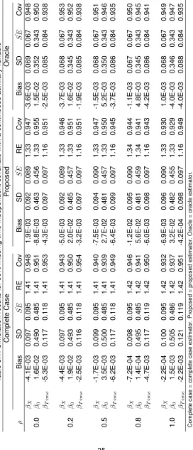
To evaluate the performance of our proposed estimator, we perform a series of simulations. We con-sider settings in which the missing and auxiliary variables are time-independent and time-varying. In addition, we let the auxiliary variable be continuous and discrete. Here we describe the simula-tions for auxiliary variables that are continuous and time-independent and discrete and time-varying. Simulations for a discrete time-independent auxiliary variable are described in Appendix B.2.

For each simulation setting, we generate longitudinal data based on the standard linear mixed-effects model in Eq. 3.1. The covariates included in the model are an intercept, time, andX, which will be missing for a subset of the sample. In addition, we include random intercepts and random slopes. Thus,Zi=γi =

1 ti

, whereti is time in years.

(38)

Sec-tion 3.2, and the oracle estimator uses the unobservable full data. Using 1000 iteraSec-tions of each simulation, we calculate the mean bias (βˆ₋β), observed sample standard deviation (SD), mean estimated standard errors (SEˆ ), mean relative efficiency (RE) compared to the oracle estimator where a lower RE is more efficient, and 95% coverage (Cov).

3.4.1. Time-Independent Missing Covariate with a Continuous Auxiliary Variable

First we describe the simulations involving a time-independent missing covariateX and a continu-ous auxiliary variableA. SinceXis time-independent, this implies thatAis also time-independent. To generate correlatedX andA, we use a standard multivariate normal distribution where(X

A)∼

Nh(µX

µA),

_σ2

X ρσXσA

ρσXσA σ2A

i

andρis the correlation betweenXandA. We simulate data forρ= 0.01, 0.25, .50, 0.75, and 1.0.

To create missing data, we first generate the full data, including the covariates, auxiliary variable, and outcome, for N=400 subjects. All subjects are considered to have observations at baseline and year one, but one-third of subjects are lost to follow-up at year two. Therefore, the data is balanced but incomplete. Then we randomly select subjects to be missing X to ensure that the missing mechanism does not depend on the auxiliary variable. We simulate data in which 25%, 50% and 75% of subjects are missingX.

Table 3.1 summarizes the results for 50% missing data. All three analyses (complete case, pro-posed, and oracle) have little bias and a good 95% coverage probability in this setting of moderate missingness. Similarly results are seen for 25% missing data (Appendix Table B.5). When the percent missing is high (75%) and the correlation between the missing and auxiliary variables is perfect (ρ=1.0), the proposed method is slightly more biased (Appendix Table B.6). Nevertheless, the mean SEˆ estimates calculated based on the asymptotic theory for the proposed estimator is similar to the observed sample SD under all conditions. As a result, the coverage probability for 75% missing data is slightly low (92%) when the correlation is high.

The RE is calculated for each estimator as ₁₀₀₀1 P1000_sim₌₁ SEˆ m,sim ˆ

(39)

complete case estimator. Moreover, even if the auxiliary variable provides little to no information aboutX, the proposed method is not necessarily equal to the complete case analysis with respect to relative efficiency. See Appendix B.1.2 for justification of this observation.

In these simulations, the RE of the proposed estimator is never 1, even for a perfectly correlated auxiliary variable (i.e.ρ= 1). This is because the proposed method does not use all of the subjects in the analysis. Instead, only those subjects in the validation set and ‘interior’ nonvalidation set are used in the analysis of the proposed method. Those subjects who are in the nonvalidation set but not the ‘interior’ nonvalidation set are not used. Thus the total sample size of the proposed method is smaller than that of the oracle method. However, in Appendix B.1.1 we show that the proposed estimator is fully efficient (i.e. RE = 1) for a perfectly correlated auxiliary variable if the sample used in the oracle analysis is restricted to be the same sample used in the proposed analysis. We should note that for a discrete auxiliary variable, the size of the oracle sample is equal to the size of the proposed method analysis sample since the ‘interior’ nonvalidation set is equal to the nonvalidation set.

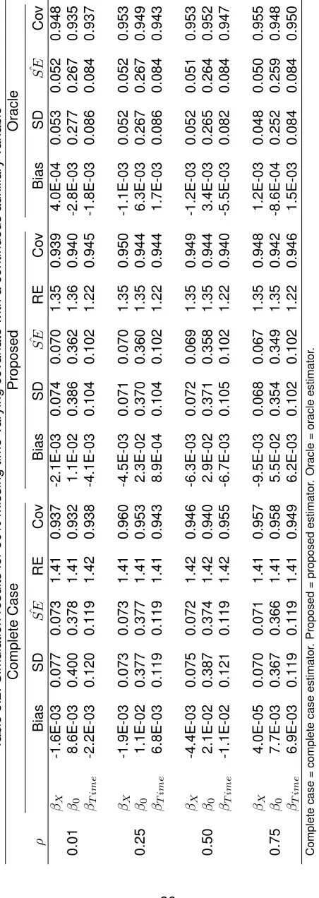
3.4.2. Time-Varying Missing Covariate with a Time-Independent Continuous Auxiliary Variable

Next, we describe the simulations involving a time-varying covariate and a time-independent con-tinuous auxiliary variable. WhenX is time-varying but Ais time-independent, we generateX in two steps. First, we generateX¯i andAi, whereX¯i is the mean forXi, from a multivariate normal

distribution whereX¯i

Ai

∼Nh(µX

µA),

_σ2

X ρσXσA

ρσXσA σ2A

i

. Second, we generateniobservations ofXi

fromNhX¯i, σ₂X

2i

. SinceX is time-varying butA is not, the correlation betweenX and Awill never be exactly 1.0. Therefore, we only consider correlations below 1. Again we set the total sam-ple size to be N=400 with one-third of subjects being lost to follow-up at year two. We also let the percent of subjects with missingX be 25%, 50%, and 75%. We evaluate the bias, efficiency, and 95% coverage probability for the three estimators forρ=0.01, 0.25, 0.50, and 0.75. In addition, we compare the efficiency of the three methods for values ofρat 0.05 increments between 0.2 and 0.75.

(40)

and correlation are 75%. As in the previous section, the small bias results in a slightly lower coverage probability of 92%. Still, the proposed method is at least as efficient, if not more, than the complete case analysis for all scenarios.

Figure 3.1 plots the RE of the complete case and proposed estimators by the percent of subjects missingX and the correlation betweenX andA. When the percent missing is below 75%, the proposed method is as or more efficient than the complete case estimate for all three correlation conditions. As the percentage of missing data increases we see more efficiency gains in the pro-posed approach when the correlation is higher.

Corr 0.25 Corr 0.5 Corr 0.75

20 30 40 50 60 70 20 30 40 50 60 70 20 30 40 50 60 70 1.25

1.50 1.75 2.00

% Missing

Relativ

e Efficiency

Method

CC

Proposed

Figure 3.1: Relative efficiency vs % missing by correlation for a time-varying missing covariate and a continuous auxiliary variable. Relative efficiency is calculated as the mean of SEˆm

ˆ

(41)

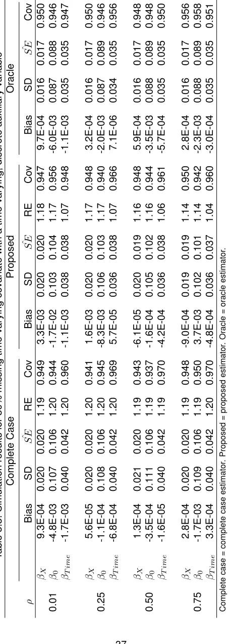
3.4.3. Time-Varying Missing Covariate with a Time-Varying Discrete Auxiliary Variable

WhenAis continuous and time-varying, the proposed estimator can be biased and inefficient, as discussed in Section 3.6. Therefore, we only consider a discrete time-varying auxiliary here. For these simulations we generate balanced and complete data with three observations for each of the N=2000 subjects. The larger sample size is necessary in these situations to have a sufficient number of validation subjects who contribute to each estimate ofPˆ(Yj|Zj). For a validation subject

to contribute to the estimate of Pˆ(Yj|Zj), the time-varying auxiliary variable must be matched at

each timepoint (i.e.I(Ai[tj] =Aj, tj⊆ti)) instead of just once (i.e.I(Ai =Aj, tj⊆ti)).

To generate data for a time-varying missing covariate and a time-varying discrete auxiliary variable, we first generate correlated continuous variables from the multivariate normal distribution described in Section 3.4.1. Since each subject has 3 observations, we generateN_×3draws from the specified distribution. Then we convertAto be a discrete variable by defining observations as 0, 1, or 2 based on the tertiles ofA. We calculate the observed correlation betweenX andAusing the Spearman correlation, which again will never be 1. In fact, the observed correlation is always smaller than the specifiedρ. Therefore, in the simulations we setρ= 0.01, 0.30, 0.57, and 0.95, to achieve the desired correlations of 0.01, 0.25, 0.5, and 0.75. We also let the percent missing be 25%, 30%, and 50%.

(42)

reasonable, one may use the baseline value, the mean, or some other summary statistic of the auxiliary variable in place of its time-varying value.

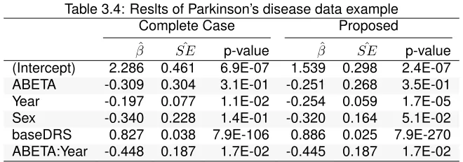
3.5. Application to Parkinson’s Disease Dementia Research

In this section, we apply our proposed method to Parkinson’s disease (PD) using the Udall Inten-sive Cohort data. This data is from an ongoing study at the University of Pennsylvania Parkinson’s Disease Center where 408 PD patients are followed longitudinally for clinical and cognitive as-sessments annually for the first four years and then biennially thereafter. Among these patients, only a fraction was randomly selected to receive extensive biomarker testing which included the measurement of CSF-aβ.

The purpose of this analysis is to understand how abnormal CSF-aβ, defined as values _≤ 192

ng/L (Shaw et al., 2009), affects the rate of change in the age adjusted Dementia Rating Scale total (DRStotalAge) in patients with PD. Since CSF-aβ values are only available for a subset of the study participants, we propose to use apolipoprotein E (APOE) genotype information as an auxiliary variable. APOE genotype information is available for most of the study participants and has been shown to be associated with CSF-aβ(Tapiola et al., 2000).

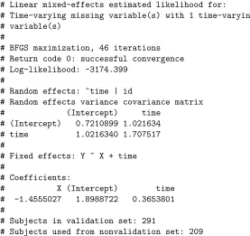
We consider the following mixed-effects model with subject-specific intercepts and slopes:

Yi=b0i+β0+β1×CSF-aβi+ (β2+b1i)×YEARi

+β3×SEXi+β4×baseDRStotalAgei

+β5×CSF-aβi×YEARi+i

(3.9)

where Yi=DRStotalAge, b ∼ N(00),

D11D12

D21D22

, and i ∼ N(0, σ2). CSF-aβi is the baseline

CSF-aβ and defined as 0 (CSF-aβ >192) or 1 (CSF-aβ _≤192). YEARi is the time from baseline

defined starting from the first recorded DRStotalAge and rounded to the nearest 6 months. SEXiis

0 (female) or 1 (male) and baseDRStotalAge_iis the baseline DRStotalAge.

Statistical Methods For Censored And Missing Data In Survival And Longitudinal Analysis

University of Pennsylvania

University of Pennsylvania

ScholarlyCommons

ScholarlyCommons

Publicly Accessible Penn Dissertations

2019

Statistical Methods For Censored And Missing Data In Survival

Statistical Methods For Censored And Missing Data In Survival

And Longitudinal Analysis

And Longitudinal Analysis

Leah Helene Suttner

Recommended Citation

Recommended Citation

Statistical Methods For Censored And Missing Data In Survival And Longitudinal

Statistical Methods For Censored And Missing Data In Survival And Longitudinal

Analysis

Analysis

Abstract

Abstract

Degree Type

Degree Type

Degree Name

Degree Name

Graduate Group

Graduate Group

First Advisor

First Advisor

ACKNOWLEDGEMENT

ABSTRACT

TABLE OF CONTENTS

LIST OF TABLES

LIST OF ILLUSTRATIONS

CHAPTER 1

INTRODUCTION

CHAPTER 2

QUANTITATIVE METHOD FOR DESIGNING APPROPRIATE LONGITUDINAL

2.1. Introduction

2.2. Motivating Study

2.3. Simulations to Study Factors Associated with Hazard Ratio Estimation Bias

Due to Right-Endpoint Imputation

2.4. Proposed Longitudinal Follow-up Evaluation Procedure

2.5. Method Validation

2.6. Application to Parkinson’s Disease Dementia Research

2.7. Discussion

CHAPTER 3

NONPARAMETRIC ESTIMATION FOR TIME-VARYING MISSING COVARIATES IN

3.1. Introduction

3.2. Proposed Nonparametric Maximum Estimated Likelihood

3.3. Asymptotic Properties of the Maximum Estimated Likelihood Estimator

3.4. Simulations

3.5. Application to Parkinson’s Disease Dementia Research