Volume 2008, Article ID 328052,14pages doi:10.1155/2008/328052
Research Article
Tracking of Moving Objects in Video Through Invariant
Features in Their Graph Representation
O. Miller,1A. Averbuch,2and E. Navon2
1ArtiVision Technologies Pte. Ltd., 96 Robinson Road#13-02, Singapore 068899 2School of Computer Science, Tel Aviv University, Tel Aviv 69978, Israel
Correspondence should be addressed to A. Averbuch,[email protected]
Received 21 July 2007; Accepted 10 July 2008
Recommended by Fatih Porikli
The paper suggests a contour-based algorithm for tracking moving objects in video. The inputs are segmented moving objects. Each segmented frame is transformed into region adjacency graphs (RAGs). The object’s contour is divided into subcurves. Contour’s junctions are derived. These junctions are the unique “signature” of the tracked object. Junctions from two consecutive frames are matched. The junctions’ motion is estimated using RAG edges in consecutive frames. Each pair of matched junctions may be connected by several paths (edges) that become candidates that represent a tracked contour. These paths are obtained by thek-shortest paths algorithm between two nodes. The RAG is transformed into a weighted directed graph. The final tracked contour construction is derived by a match between edges (subcurves) and candidate paths sets. The RAG constructs the tracked contour that enables an accurate and unique moving object representation. The algorithm tracks multiple objects, partially covered (occluded) objects, compounded object of merge/split such as players in a soccer game and tracking in a crowded area for surveillance applications. We assume that features of topologic signature of the tracked object stay invariant in two consecutive frames. The algorithm’s complexity depends on RAG’s edges and not on the image’s size.
Copyright © 2008 O. Miller et al. This is an open access article distributed under the Creative Commons Attribution License, which permits unrestricted use, distribution, and reproduction in any medium, provided the original work is properly cited.
1. INTRODUCTION
Object tracking is an important task for a variety of computer vision applications such as monitoring [1], perceptual user interfaces [2], video compression [3], vehicular navigation, robotic control, motion recognition, video surveillance, and many more. These applications require reliable object tracking techniques that satisfy real-time constraints. For example, object tracking is a key component for efficient algorithms in video processing and compression for content-based indexing [4,5]. In MPEG-4, the visual information is organized on the basis of the video object (VO) concept, which represents a time-varying visual entity with arbitrary shape. Tracking these video objects along the scene enables individual manipulation of its shape and combines it with other similar entities to produce a scene.
A robust tracking system should meet the following challenges: tracking of multiple objects that are partially covered (occluded) by other objects, tracking a compounded object of merge and split as players in a soccer game, tracking of slow disappearance of an object from a scene and then
Producing an automatic robust tracking system is a significant challenge. There have been a lot of efforts that produce solutions to handle the tracking problem. The existing techniques in the literature can be roughly classified into the following groups of trackers: region-based, contour-based, and model-based.
1.1. Region-based trackers
An adaptive algorithm, which updates the histogram of the tracked object in order to account for changes in color, illumination, pose, and scale, was presented in [7]. The tracked object is represented as “blobs” in the back-projection [8]. This technique has a low complexity, and thus suits real-time systems. Other techniques, which utilize structural features such as texture, color and luminance, are proposed in [9–11]. For example, [9] suggested a moving object tracking algorithm that is based on a combination of adaptive texture and color segmentation. They use Gibbs-Markov random field to model the texture, and a two-dimensional Gaussian distribution to model the color. The tracked target is obtained by a probabilistic framework of the texture and color cues at region level and by adapting both the texture and color segmentation over time. Similar techniques were used earlier in [10,11]. However, when fast motion of the object and significant change in behavior are allowed, color- or texture-based techniques are not sufficient to detect a long-term tracking. Region-based algorithms to deal with the above were suggested in [12,13]. The method in [12] is based on a modified version of Kalman’s filter. A four-step tracking technique using motion projection, marker extraction, clustering and region merging was suggested in [13]. The motion projection represented by a linear motion model is calculated on the reliable parts of the projected object. These parts are called marker points and their extractions are based on the assumption about the relationship between the projected and real objects. Then, starting from these markers, a modified watershed transfor-mation followed by a region-merging algorithm produces the complete segmentation of the next frame. The advantage of the techniques in [12,13] is in their abilities to deal with significant changes in the object’s regions.
1.2. Contour-based trackers
These algorithms detect and track only the contour of the object. For example, the snake algorithm [6] does it by using a converged snake in the reference frame as the initial snake in the successive frame. However, the algorithm blurs the image to disperse gradient information. Therefore, it has a limited search area and it is unable to track changes in the contour that lie outside the range of the blurred gradient operator. As a consequence, this method is effective only when the motions and changes in the object’s shape between consecutive frames are small. To overcome this limitation, some use dynamic programming that increases the search area of the snake. Temporal information to bias the snake toward the shape of the segmentation in the previous frame is used in [14]. This method improves the shape memory
of the snake but does not adequately track large-scale object movements or significant changes in its shape. Conversely, [15] suggested a tracker, which handles significant changes in the shape. It partitions the object’s contour into several curves and estimate the motions of each curve independently of the others. Then, the predicted location of the complete contour is obtained by using dynamic programming. A particle filter-based subspace projection method, which neither causes blur nor demands an expensive dynamic programming, is presented in [16].
1.3. Model-based trackers
A generic solution to object tracking is still a challenging problem. Therefore, model-based techniques, which demand a priori information regarding the object’s shape and type, were developed for suitable applications. For example, [17] suggested a model, which is based on edge detector, to extract moving edges that are grouped together by a predefined model shape. A similar concept was used in [18], which groups the edges by using the Hough transform. In addition, the use of deformable templates has been very common in model-based techniques. A deformable template enables to track large movements and changes, and also provides global shape memory for the tracked object. For example, a known model of a key is defined in [19]. This approach allows both affine transformations of the entire key and local deformations in the form of variations in the notches of the key. A similar approach of deformable templates was used in [20] for tracking a human hand by global and local deformation templates, which were defined for movement changes and for finger motions, respectively. Recently, a dynamic-model-based technique [21], which decreases the constraint limitation by having a predefined model, was suggested. It uses a hierarchy of separate deformation stages: global affine deformations, local (segmented) affine deformations, and snake-based continuous deformations. This approach provides a shape memory update of the object’s model and thus, enables the snake algorithm to be used for final contour refinement after each frame.
Our proposed algorithm is classified as a contour-based technique. The algorithm gets as an input the contour (curve) of the moving object to be tracked and two consecutive framesItandIt+1in timestandt+1, respectively.
Initially, we apply a still-segmentation process onItandIt+1.
Region adjacency graphs (RAGs), denoted byGt andGt+1,
are the constructed data structures from the segmentation of It andIt+1, respectively. Then, the contour of the extracted
object in Gt is segmented into subcurves while interior
junctions are marked. Each subcurve represents a different homogeneous region inGt. The interior junctions connect
between two different subcurves. These junctions are called important (easy) points to track. Motion estimation of these junctions is performed where the search area is the edges in Gt+1. For each pair of tracked junctions in Gt, there
exists a small number of “candidate paths,” which connect the estimated pair inGt+1. These paths are obtained by an
the candidate paths accurately represents the single-tracked subcurve between a pair of junctions. Then, the construction of the tracked object is actually a process that matches between a single edge (signature) inGtand a set of candidate
paths inGt+1.
The matching process has a low complexity due to the limited number of candidate paths. The tracked contour is constructed from all the matched paths between pairs of estimated junctions. We show that the probability of matching the right path is proportional to the number of points that participate in the matching process.
In contrast to other contour-based techniques such as in [6,14,15], our algorithm does not use the snake algorithm [6] to obtain the predicted curve of the object. Therefore, the suggested algorithm does not have limitations on the object’s motion or changes in the object’s pose. Furthermore, it does not require a priori information about its shape, type, or motion as in [17,19,20].
The rest of the paper is organized as follows.Section 2 introduces the notation and outlines the main steps of the algorithm. Section 3 describes the object’s contour segmentation. The estimation of the junction’s motion and the algorithm for finding the candidate paths is given in Section 4.Section 5presents the matching process that con-structs the tracked contour. Implementation and complexity analysis is given inSection 6. Experimental results are given inSection 7.
2. NOTATION AND OUTLINE OF THE ALGORITHM
The following notations are used; see Figure 1 for illus-tration. The flow of the algorithm is given in Figure 2. Let It and It+1 be the inputs of the source frame and its
consecutive frame, respectively. We denote by {Rti},i =
1,. . .,nt and{Rtj+1}, j = 1,. . .,nt+1 the sets ofnt andnt+1
non-overlapping regions that are generated by a still image segmentation (Section 3.1 using [22–24]) of It and It+1,
respectively. Region adjacency graphs (RAGs)Gt =(Vt,Et)
andGt+1=(Vt+1,Et+1) are the data structures that represent
the segmentation ofIt andIt+1, respectively. The nodes of
the RAGs represent the regions Rti,i = 1,. . .,nt. An edge
e(i,j)∈Etrepresents a shared common boundary ofRtiand
Rtjsuch that (x,y)∈e(i,j), for all (x,y)∈Rti∩Rtj. The same
is true forGt+1=(Vt+1,Et+1).
Let Ct be the closed input curve that belongs to the
object’s contour to be tracked inItsuch thatCt ⊆Etand let
Ct+1 be the tracked contour inIt+1. We assume thatCt+1 ⊆
Et+1. The “important” points inCt are calledjunctions(see
Section 3.2). They are denoted byJk, k=1,. . .,N, which is
the set of theNjunctions on the curveCt. Thus,Ct(source) is
segmented into subcurves, denoted byPkt,k+1, k =1,. . .,N,
where the indices that enumerate the junctions are k =
1,. . .,N−1 and theNth junction is connected to 1. Each subcurvePtk,k+1is actually the edge that connects the pairJk
andJk+1. The corresponding points of Jk, k = 1,. . .,N in
It+1are denoted bySk, k=1,. . .,N, such that each matched
point inSk corresponds to a junction inJk. In other words,
a set of matched points in Jk, k = 1,. . .,N, inIt+1 will be
detected by a block-matching process (Section 4.1) that is based on SAD minimization of the matched squared errors betweenJk, k=1,. . .,N, and a searched area inIt+1. The set
of matched points inIt+1isSk, k=1,. . .,N.
The construction ofCt+1 is achieved by the application
of the matching procedure (Section 5.1) that measures the similarity between the edges of It and It+1. We will show
(Section 5.1) that each subcurve inCt (the edge betweenJk
andJk+1) has a single matched edge inCt+1 (the edge that
connectsSk andSk+1). However, several edges may connect
the matched pointsSk and Sk+1. We call this set of edges
“candidate paths” (destination), denoted by Pkt+1,k+1, r =
1,. . .,Rk, whereRkis the number of candidate paths between
eachJk andJk+1. We say thatCt+1 ⊆ Ptk+1,,k+1r,r = 1,. . .,Rk.
There exists rk, 1 ≤ rk ≤ Rk, such that a path Pkt+1,,k+1rk that
satisfiesPkt+1,,k+1rk ∈ Ct+1 is called amatched path, denoted by mptk+1,k+1. Then,Ct+1= ∪k=1,...,N−1mpkt+1,k+1. In other words, the
new object’s curveCt+1 is formed by sets of matched paths
mptk+1,k+1betweenSkandSk+1, k=1,. . .,N.
3. CURVE SEGMENTATION
Assume we have the two input frames It andIt+1 and an
object’s contour Ct. Segmentation of the object’s contour
(curve) Ct into subcurves is required since the object may
translate and rotate in three-dimensional space, while its projection onto the image plane causes substantial deforma-tions in its two-dimensional shape. Therefore, it is better to estimate separately the motion of each subcurve rather than estimating the motion of the entire object’s contour. The segmentation of the object’s contour into subcurves is achieved by finding a set of junctions, which connect the subcurves between themselves and separate between homogenous regions. In (Section 3.2), we justify why these junctions are well-tracked points that faithfully represent the rest of the points that belong toCt. These junctions comprise
the signatureof the tracked object that will characterize it uniquely.
In order to partition the object’s curve into subcurves, we utilize the still-segmentation results ofIt. We require from
the still segmentation to produce homogeneous regions such that only the boundaries of the regions overlap each other.
3.1. Image segmentation
The performance of the algorithm is directly affected by the number of segments from the two input framesIt andIt+1.
We want produce a minimal number of segmented regions while preserving the homogeneity criteria. For this purpose, we apply the segmentation algorithm in [22–24].
R11
R14
R8
R6
R10
R1
R13
R4
R2
R12
R3
R5
(a) (b)
Figure1: (a) Still segmentation ofIt.Ct(source) is the green closed curve. The red contours are the segmented boundaries. The black arrows
point to two different junctionsJ1andJ2. (b) Still segmentation ofIt+1.Ct+1is the tracked green closed curve and the black arrows point to
the matched pointsS1andS2that correspond to the junctionsJ1andJ2, respectively. The yellow curves are the paths ofPt1,2+1,r,r =1,. . ., 3
and the blue curve is the matched path denoted bymp1,2
t+1.
It Ct It+1
Ct+1
Curve segmentation Segmentation ofItandIt+1
Detection of junction inCt
Finding candidates paths Estimating the matched points
inIt+1to junctions inCt
Finding candidate paths between estimated junctions
Construction of the tracked curve
Figure2: Flow diagram of the proposed algorithm whereIt and
It+1are two consecutive input frames, andCtis the input object’s
contour to be tracked.Ct+1is the tracked contour inIt+1.
the image is divided into lakes. Each lake represents a region. However, due to its sensitivity to weak edges, the watershed algorithm generates oversegmented output. Therefore, its output is used as an initial guess for the merging process phase, which aims at reducing the number of segments. The
merging process is done iteratively. At any iteration during the merging process, the most similar adjacent regions are merged. The similarity between any pair of adjacent regions is measured by the outcome of a dissimilarity function [22– 24]. Local thresholds are derived by an automatic process, where local information is taken into consideration. Any threshold refers to a specific region and its surroundings. The number of thresholds that defines the final regions is known only when the process is terminated. The output of the segmentation is represented by Rt
i, i = 1,. . .,nt,
which partitions It. These partitions construct the initial
data structures that we use during the entire duration of the algorithm. Recall that Gt = (Vt,Et) (Section 2) is an
undirected graph that represents the partition of It. The
region Rti is represented by a nodevi ∈ Vi. An edgee(i,j)
exists only ifRtiandRtjare adjacent, where adjacent regions
share a boundary. The edgee(i,j) contains all the pixels that lie betweenRtiandRtj. Hence, all the pixels of the segmented
boundaries are represented byEt. The same is true for the
graphGt+1=(Vt+1,Et+1).
3.2. Detection of a junction
The proposed algorithm first tracks the “important” points (junctions)Jk, k = 1,. . .,N. We will show here that these
points are sufficient to produce reliable tracking without the need to have the rest of the points inCt.
The algorithm mainly detects corners as well-tracked points. Hence, corners are considered important points to track.
A corner is defined as a meeting point of two (or more) straight edge lines [26–29]. Following this definition, each corner contains at least two different edges and at least two different regions, which together create two-dimensional structures. Since real images do not contain geometric shapes only or rigid objects, corners are related to curvature on the contour. L-junction, T-junction, and X-junction are different corner types, where the number of regions that meet in the corner determines the corner type. Examples of a T-junction profile and corners in a synthetic image are illustrated in Figure 3.
The corners, as a source for rich information, are used as an anchor points for tracking. Corners can be tracked with high accuracy as it is demonstrated in [26,30]. In [31,32] corner tracking is used for robot homing and low bit rate video codec, respectively.
Since corners are well-tracked points, we are motivated to associate the important points inCtwith corners. Hence,
the important points (which are called junctions) are defined as follows.
Definition 1. Let Ct be the contour of a given object. Let
Rtk, k = 1,. . .,N, be the subset ofRti, i = 1,. . .,nt, which
is represented byGt =(Vt,Et). AssumeN(N≤nt) regions
of the object intersect Ct. The N regions are renumbered
1,. . .,N such that Rtk is adjacent to Rtk−1 and Rtk+1 for all
k=1,. . .,N. A junctionJk, k=1,. . .,N, onCtis defined as
Jk=Δ(x,y), where (x,y)∈Ctand (x,y)∈e(k,k+ 1), e∈Et.
In other words, a junction is defined as a point onCt
where two interior segments of the object meet. Junctions are distinguished from corners by the fact that they are not necessarily represented as a meeting point of straight lines and do not necessarily represent a curvature inCt (see
Figure 4). However, like corners, junctions contain at least two different edges (lines). They represent a meeting point of at least two different homogenous regions of the object, while a corner may represent only homogeneous region of the object. They are considered as good features and are used in our application as “important” anchor points to base the tracking on them.
4. FINDING THE CANDIDATE PATHS
InSection 3, we discussed the advantages of having junctions inCtas well-tracked points. The junctions enable to find a set
of matched pointsSk, k=1,. . .,NinIt+1and the candidate
pathsPtk+1,,k+1r, r=1,. . .,Rkfor the construction ofCt+1.
The construction of the object’s contour Ct+1 in
It+1 relies on the fact that the set Jk, k = 1,. . .,N,
is defined as connected points between homogeneous regions in Ct (see Figure 4). Any pair of
consecu-tive junctions Jk and Jk+1 is connected by a subcurve
Ptk,k+1. This subcurve is an edge in Gt that represents
the boundary of a homogeneous region. As defined in Section 2, Sk, k = 1,. . .,N, is a set of matched points
Gray level 1
Gray level 2 Gray level 3
(a) (b)
Figure3: (a) Profile of T-junction. (b) Corner map (red dots) of a synthetic image.
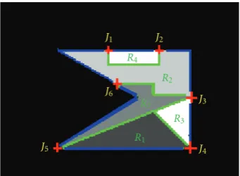
J1 J2
J3
J4 J5
J6
R1 R3
R5
R2 R4
Figure 4: Syntactic illustration of detected junctions inCt. The
blue curve is the object contourCt. Each homogeneous region in
Ctis bounded by a green curve. The red crosses onCt represent
a set of six junctionsJk, k = 1,. . ., 6. Each connection between
two consecutive junctionsJk andJk+1, represents a homogeneous
region. Each junctionJk, k=1,. . ., 6 is a connection between two
(or more) segmented regionsRiandRj,i,j=1,. . ., 5 andi /=j. The
two top corners are the curvature regions ofCtthat do not satisfy
Definition 1.
(inGt+1) to set Jk, k = 1,. . .,N (inGt). Each consecutive
pairSkandSk+1can be connected by several paths which are
edges inGt+1 (seeFigure 1). However, based on our image
segmentation assumption, the contour of the tracked object Ct+1 is an integral part of the segmentation outputs such
that Ct+1 ⊆ Et+1. Since all possible paths betweenSk and
Sk+1, k = 1,. . .,N, satisfyEt+1 = ∪k=1,...,N,r=1,...,RkP
k,k+1 t+1,r we
get that Ct+1 ⊆ ∪k=1,...,N,r=1,...,RkP
k,k+1
t+1,r. After these sets of
paths (candidate paths) between each pair inSkare obtained,
the construction of Ct+1 is done by the application of the
matching process between a single edge Ptk,k+1 to the set
Ptk+1,,k+1r, r = 1,. . .,Rk. These paths mean that we actually
transform the tracking of the entire curve into a problem of how to identify match between edges.
This section describes how to find the matched pointsSk
forJk, k =1,. . .,NinEt+1(Section 4.1). Then, we describe
the algorithm that finds candidate pathsPtk+1,,k+1r, r=1,. . .,Rk
4.1. Finding the corresponding junctions
The match between regions in consecutive frames is done by the application of a block-matching process on the set of junctionsJk, k =1,. . .,N. This set contains information
about the connected points between the object regions Rti, i = 1,. . .,nt, that intersect Ct. Although we assume
nothing about the object’s motion, the overall structure of the object is generally preserved between two consecutive frames. The interior regions of the object do not radically change and so their connecting points. Therefore, the information that is stored in Jk, which is contained inEt,
should also exist in the object’s boundaries inEt+1.
Unlike traditional motion estimation techniques, where the search area is usually a predefined squared window, we utilize the data structure of Gt+1 to adaptively determine
the search area of each point inJk, k = 1,. . .,N. The still
segmentation ofIt+1enables to define the set of pixels in the
edgesEt+1of the RAGGt+1as the search area for finding the
corresponding matched pointSk. Thus, only a small portion
of the whole image participates in the search process (block matching), which reduces the complexity (O(|Et+1|)) to be
dependent only on the graph edges.
The center of the search window is located in the coordinates of each Jk, k = 1,. . .,N. Our goal is to find
the motion vector that minimizes the matching error for a given junctionJk. It is being done through a common block
matching procedure. The matching error between the block that is centered in (xk0,y0k)∈Jkand has a matched pointSkis
SAD(x,y)
xk0,yk0
= B/2
j=−B/2 B/2
i=−B/2 It
xk 0,yk0
−It+1
x+i,y+j, (1)
whereB×Bis the block size. Among all the searched points in (x,y) ∈ Et+1, the matched point is assigned toSk, k =
1,. . .,Nthat minimizes the matching error score
Sk=Δarg min (x,y)∈Et+1
SAD(x,y)
xk 0,y0k
. (2)
The SAD(x,y)(xk0,y0k) is computed for eachJk, k =1,. . .,N.
Then, we obtain the set ofmatched pointsSk, k =1,. . .,N.
Figures8(c)and8(d)illustrate the setsJk, Sk, k=1,. . .,N,
respectively. We anticipate thatSk ⊂ Ct+1 fork = 1,. . .,N.
Therefore, the curveCt+1 of the tracked object is assumed
to pass through the matched points. If only one curve passes through the matched junctions, the algorithm is terminated and this curve is considered as the object’s contourCt+1. However, this is not always the case in real and
inhomogeneous images. Several curves may pass through each pair of the matched points (seeFigure 1). Section 4.2 describes how to find these curves, based on the algorithm that finds thekshortest paths between two nodes in a given graph.
4.2. Finding thekshortest paths (candidate paths)
The RAGGt+1 is transformed into a connected and
undi-rected weighted graph Gt+1 = (Vt+1,Et+1) as follows.
Initially, any pixel (x,y)∈Et+1 is represented by a node in
Gt+1. In other words, each pixel on the boundaries of the
segmentation is a node inGt+1. Every two nodes inGt+1are
connected by an edge e ∈ Et+1 if they are adjacent. Thus,
Gt+1is another representation of the segmentation whileGt+1
focuses on regions and their connections, andGt+1 focuses
on the boundaries of the segmentation. Since the matched points satisfySk⊆Et+1, they are nodes inGt+1. Consequently,
all the pathsPkt+1,,k+1r, r =1,. . .,Rk, betweenSkandSk+1, that
have to be found, are exactly the paths inGt+1betweenSkand
Sk+1.
Assume that Gt+1 is a connected graph. Then, at least
one path exists between any pair of nodes. The numberRk
of paths between two given nodesSk andSkinGt+1 can be
big. Since the length ofmptk+1,k+1has to be approximately the
length of the source pathPkt,k+1, we define Lk,k+1 to be the
maximal length of the candidate pathsPtk+1,,k+1r, r =1,. . .,Rk.
Lk,k+1 is initialized to be twice the length ofPtk,k+1. Hence,
findingPkt+1,,k+1r, r =1,. . .,Rk, which are shorter thanLk,k+1, is
equivalent to the problem that lists all the paths that connect a given source-destination pair in a graph shorter than a given length.
The proposed algorithm is based on [33] that finds the k shortest paths. Thek shortest path algorithm lists k paths, which connect a given source-destination pair in a directed graph with minimal total length. The main idea is to construct a data structure from which the sought after paths can be listed immediately by focusing on their unique representation. The data structure is constructed by handling separately the edges of the shortest-path-tree from those which are not. By differentiating between the edges, any path can be represented only by edges, which are not in the shortest-paths-tree. In addition to the implicit representation of a path, any path can be represented by its father and an additional edge. The father of a path differs from it only by one edge, which is the last edge among all the edges that are not in the shortest-paths-tree. An order-path-tree is constructed from this representation and the sought-after paths are constructed through its use. Before we describe the construction of the data structure we transformGt+1by this technique, which is described in [34],
to become a directed graph denoted byGt+1 =(Vt+1,Et+1).
The direction of the sought-after paths is fromSktoSk+1.
We denote byhead(e) andtail(e) the two endpoints of an edgee∈Et+1, which is directed fromtail(e) tohead(e).
The length of an edgeeis denoted byl(e). An example of a directed graph with lengths attached to its edges is shown inFigure 5(a). The length of each edge inGt+1is initialized
to 1. The length of a path p ∈ Gt+1, which is the sum
of its edge lengths, is denoted by l(p). The length of the shortest path from Sk to Sk+1 is denoted by dist(Sk,Sk+1).
We find the shortest path from each vertex v ∈ Gt+1 to
Sk+1. The set of all these paths generates a single-destination
shortest path tree, denoted byT(seeFigure 5(b)). From the construction of T, the edges in Gt+1 are divided into two
s
t
2 20 14
9 10 25
18 8 11
13
15
27
20
14
12
15
7
(a)
55 56 36 22
42 33 23 7
37 19 11 0
(b)
s
t
3
9 10
4
6
1
(c)
{}
{3} {6} {10}
{3, 1} {3, 4}
{3, 1, 9} {3, 4, 6} {3, 4, 9}
(d)
Figure5: (a) A directed graphGwith different edge lengths. The nodes which are marked by “s” and “t” are the sourceskand destination
sk+1, respectively. (b) The single-destination shortest path treeT. (c) The values ofδ(e) of all the edges inG−T. (d) The order path tree is
constructed by the father-son representation while only sidetracks are used.
measures the difference between dist(tail(e),Sk+1) and the
shortest path fromtail(e) toSk+1 that contains e. In other
words,δ(e) measures the lost distance caused by addingeto the shortest path.δ(e) is defined as
δ(e)=Δl(e) + disthead(e),Sk+1
−disttail(e),Sk+1
. (3)
Then, for anye ∈T, we get thatδ(e)= 0 and for anye ∈
Gt+1−T, δ(e) > 0. We call the edges withδ(e) > 0 (the
edges in the second group) “sidetrack” edges. Examples of all e∈Gt+1−Tand theirδ(e) values are shown inFigure 5(c).
Any pathp ∈ Gt+1 is described by a sequence of edges
that contains edges inTand sidetrack edges. Listing only the sidetracked edges was found to be a unique representation of psince every pair of nodes, which are the endpoints of two successive sidetrack edges inp, is uniquely connected by the shortest path between them (from edges inT). Ifpdoes not contain sidetracks,pis the shortest path inT. Consequently, the length of p, which connects the nodes SkandSk+1, can
be computed as the sum of dist(Sk,Sk+1) and the length of its
sidetracks. From the fact that any path can be represented only by its sidetracks, an additional interpretation can be used. Let prepath(p) be the sidetracks of p except for the last one. We call the path, which is defined by the set of prepath(p), the father of p. Any path p with at least one sidetrack can be represented by its prepath(p) and by its last sidetrack. From the father-son relation, we can construct an order-path-tree (seeFigure 5(d)) in which all the paths in Gt+1 are represented. The order path tree contains only the
edges in Gt+1 −T since the edges in T are already stored
in an appropriate data structure (which isTitself) that fits
the implicit representation. This data structure, which is described next, is constructed from different heaps into a final graph. All the pathsPkt+1,,k+1r, r =1,. . .,Rk, in Gt+1 will
be represented by paths from the final graph.
We denote each vertexv∈Gt+1by out(v) of the edges in
Gt+1−Twith a tail inv. For eachv∈Gt+1, we construct a
heapHout(v) from the edges in out(v). Each node inHout(v)
has at least two sons, while the root has only one.HT(v) is a
heap ofvthat contains all the roots ofHout(w), wherewis on
the path fromvtoSk+1.HT(v) is built by merging the root of
Hout(v) intoHT(nextT(v)), where nextT(v) is the next node
that follows aftervon the path fromvtoSk+1inT(Figure 6).
We formedHG
t+1(v) by connecting each nodewinHT(v) to
the rest of the heapHout(w) except for the two nodes it points
to inHT(v). By merging allHGt+1(v) for eachv∈G
t+1, we get
a direct acyclic graphD(Gt+1) (seeFigure 7(a)). We denote by
h(v) the root ofHGt+1(v) and useδ(v) instead ofδ(e), where eis the edge inGt+1that corresponds tov.
D(Gt+1) is augmented to thepath graph, that is denoted
by P(Gt+1) (see Figure 7(b)). The nodes of P(Gt+1) belong
to D(Gt+1) with the rootr = r(Sk) as an additional node.
The nodes of P(Gt+1) are unweighted but the edges are.
Three types of edges exist in P(Gt+1). (1) The first type is
the edges inD(Gt+1). Each (u,v) has a lengthδ(v)−δ(u).
(2) The second type is the edges from v to h(w), where v ∈ P(Gt+1) corresponds to an edge (u,v) ∈ Gt+1 −T.
These edges are calledcross-edges. (3) A single edge betweenr andh(w) with lengthδ(h(Sk))represents the third type. From
3∗ 6∗ 10 9∗
1∗ 4∗
1∗
6∗ 10∗ 9∗
6∗ 9∗
9∗
Figure6:HT(v) of each node inGinFigure 5(a), where out(v) is
not empty. For anyv ∈ GinFigure 5, out(v) contains only one node, therefore,HG(v) is equal toHT(v).
s· · · 3
d· · · 6
e· · · 6
f· · · 9
a· · · 1
b· · · 1
6 9
10
9
4
(a)
r
3
3 3
1 7
4 3
3
9 3
6 9
(b)
Figure7: (a)D(G). It has a node for each node that is marked
by (∗) in Figure 6. The nodes that are marked by (∗) are the nodes that were updated by the insertion of the root of out(v) into HT(nextT(v)). (b)P(G).
paths fromSk toSk+1 ∈ Gt+1. To prove this claim, we have
to show that any pathp ∈Gt+1 corresponds to a pathp ∈
P(Gt+1) that starts fromr, and any pathpfromr∈P(Gt+1)
corresponds to a pathp ∈Gt+1, which is represented by its
sidetracks.
Next we outline the proof that any path p fromr ∈
P(Gt+1) corresponds to a pathp∈Gt+1. We list for any path
p ∈ P(Gt+1) a sequence of sidetracks, which represents its
corresponding pathp∈Gt+1, as follows. For any cross-edge
in p, the edge inGt+1, which corresponds to the tail of the
cross edge, is added to the sequence. The last edge added is the edge inGt+1 that corresponds to the last vertex in p.
Since each node inP(Gt+1) corresponds to a unique edge in
Gt+1−T, the sequence of edges, which is formed to represent
p, consists only of sidetrack edges.
Given the representation of all paths inGt+1, we construct
the heap H(Gt+1) in order to list only the sought-after
paths, which are shorter than the given threshold.H(Gt+1)
is constructed by forming a node for each path inP(Gt+1)
rooted atR. The parent of a path is the path that is achieved by the removal of the last sidetrack. The weights of the nodes
are the length of the paths. From the construction, each son is shorter than its father, and the weights are heap-ordered.
Finally, we apply the length-limited depth first search (DFS) [27] on H(Gt+1). The length-limited DFS is the
regular DFS algorithm with the following modification. If the weight of the current node is bigger than Lk,k+1, the
process is regressed and continues with the node that was reached before the current node. The search results are the set of nodes that reached weights smaller thanLk,k+1. Then,
we translate the search results to a full description of the paths with the representation discussed above (any path is described as a sequence of edges inTand edges inGt+1−T).
This translation generates all the candidate pathsPkt+1,,k+1r, r =
1,. . .,RkbetweenSkandSk+1, that are shorter thanLk,k+1.
5. CONSTRUCTION OF THE TRACKED CONTOUR
We claim that there exists a strong similarity between mptk+1,k+1 ⊆ Ptk+1,,k+1r,r = 1,. . .,Rk, and the original (source)
pathPtk,k+1 inCt. This similarity exists due to the fact that
the segmentation of the contourCtrepresents homogeneous
subcurves (edges)Ptk,k+1, k =1,. . .,N(Section 3.2), by the
homogeneity criteria. Homogeneous subcurves in Ct are
likely to preserve their contents between consecutive frames. Furthermore, the candidate path Ptk+1,,k+1r, r = 1,. . .,Rk,
represents different homogeneous edges (see Section 3.1). Thus, even if the content of the edge is changed such that Ptk,k+1 becomes different from mpkt+1,k+1, it is unreasonable
thatPtk,k+1will transform its content to be similar to one in
Ptk+1,,k+1r −mptk+1,k+1,r=1,. . .,Rk.
We are given the candidate pathsPkt+1,,k+1r, r = 1,. . .,Rk,
k = 1,. . .,N. The construction of the tracked curveCt+1 is
transformed into a process that matches between the edges. The tracked contourCt+1will be constructed by the matched
pathsmpkt+1,k+1, k=1,. . .,N, which are independent of each
other. All its candidate paths Pkt+1,,k+1r, r = 1,. . .,Rk between
each pair of successive pointsSkandSk+1are listed. Then, the
path which is the most similar path toPtk,k+1(the connection
between Jk and Jk+1) among all Ptk+1,,k+1r, r = 1,. . .,Rk, is
considered as thematched pathmpkt+1,k+1∈Ct+1.
5.1. Match between paths
The process that findsPtk+1,,k+1r, r =1,. . .,Rk,k =1,. . .,N, is
based only on the segmented boundaries. On the other hand, the detection of the matched paths mpkt+1,k+1 is performed
using the original input contourCt. SincePkt,k+1is composed
of one homogeneous region, not all its points are needed in the matching procedure.
LetSPtk,k+1be a subset ofβindependent points inPtk,k+1.
A search for the best match between any pixel (x,y)∈SPtk,k+1
and all the pixels in Ptk+1,,k+1r, r = 1,. . .,Rk, is performed.
A matched grade is computed for every (x,y) ∈ Ptk+1,,k+1r,
r = 1,. . .,Rk, using (1). The matched value is assigned to
(a) (b) (c)
(d) (e) (f)
Figure8: Step-by-step illustrations of the main steps of the algorithm. (a) and (b) are the input frames. (c) and (d) illustrate the junction detection with their matched points, respectively. (e) illustrates a single set of candidate paths, and (f) is the final tracked object.
Sf
(
p
)
0 5 10 15 20 25 30 35 40
Sample size (%)
20 50 80 100
Path1 Path2
Path3 Path4
Figure9: The values ofS fk(p) (6) as function ofβ(sample size) for
the four paths inFigure 8(e).βis assumed to be 20%, 50%, 80%, and 100%.
pixels (x,y)∈Ptk+1,,k+1r,r =1,. . .,Rk. We call this point thebest
pointand denote it bybpkt+1,k+1(x,y). In addition,BPkt+1,k+1(x,y)
denotes the set of all thebest point that corresponds to the subsetSPtk,k+1. Then, fork=1,. . .,N, we have
BPtk+1,k+1=
bptk+1,k+1(x,y)|(x,y)∈Pkt+1,,k+1r, r=1,. . .,Rk
. (4)
If BPtk+1,k+1 belongs entirely to a single path p, p ∈ Pkt+1,,k+1r,
r = 1,. . .,Rk, such that BPtk+1,k+1 ⊆ p, then this path is
considered as the matched pathmpkt+1,k+1 inCt+1. Otherwise,
we differentiate between the paths by giving a grade to each p∈Ptk+1,,k+1r,r =1,. . .,Rkas follows. Fork=1,. . .,Nand for
each (x,y)∈Ptk+1,,k+1r,r=1,. . .,Rk, the characteristic function
fk(x,y) is defined as follows:
fk(x,y)
Δ
= ⎧ ⎨ ⎩
1, (x,y)∈BPtk+1,k+1,
0 otherwise. (5)
Each path p ∈ Pkt+1,,k+1r, r = 1,. . .,Rk is assigned with a
matched gradeS fk(p) by
S fk(p)=Δ
(x,y)∈p
fk(x,y). (6)
Then, we consider the path that maximizes S fk(p) as the
matched pathmpkt+1,k+1:
mpkt+1,k+1
Δ
= arg max
p∈Pk,k+1 t+1,r,r=1,...,Rk
S fk(p). (7)
Although not all the best points satisfyBPtk+1,k+1 = mptk+1,k+1,
most of them do. The use of a set of best points in each subcurve Ptk,k+1 is aimed to offset and correct the errors
produced by the minimization of the SAD measurements of a single point. However, since the searched area{(x,y) : (x,y) ∈Ptk+1,,k+1r, r =1,. . .,Rk}is characterized by different
(a) (b) (c)
(d) (e) (f)
Figure10: Final tracking results for five successive frames taken from “Stefan” video sequence.
bpkt+1,k+1(x,y) to reside either inCt+1or in a relatively far and
dissimilar region. Note that the grades, which distinguish between the path mpkt+1,k+1 and the other paths Pkt+1,,k+1r −
mptk+1,k+1, r = 1,. . .,Rk, are affected by the subset size β.
Decreasing the size of β reduces the computational time, especially for longer paths. Subset paths ofβ = 30% from the original subcurvePkt,k+1are sufficient to reliably produce
the contourCt+1.
6. IMPLEMENTATION AND COMPLEXITY
Our method stresses the accuracy in finding the object’s contour and not the area where it is located. An efficient implementation is achieved while preserving the accuracy of the final results.
6.1. Implementation
input:It,Ct,It+1
output:Ct+1
process:
(1) Still segmentation in Section 3.1that uses [22–24] is applied on It and It+1.Rti, i = 1,. . .,nt andRtj+1, j =
1,. . .,nt+1are the segmentations ofItandIt+1, respectively.
(2)Gt=(Vt,Et) andGt+1=(Vt+1,Et+1) are constructed.
They represent the segmentation ofItandIt+1, respectively.
(3) For every (x,y)∈Ct, we check whether (x,y) satisfies
the junction definition. If it does, we add (x,y) to the set of junctionsJk, k=1,. . .,N.
(4)Ctis segmented intoPtk,k+1, k = 1,. . .,Nsubcurves
that correspond to the set of junctionsJk, k=1,. . .,N.
(5) For every junctionJk, k=1,. . .,N, do the following.
(a) Its SADs (1) are calculated in the corresponding searched area inEt+1.
(b) The point with the minimal SAD 2 is added to Sklist.
(6) The graphGt+1is constructed fromGt+1.
(7) For everySkandSk+1, k=1,. . .,N, do the following.
(a) All the candidate paths Pkt+1,,k+1r, r = 1,. . .,Rk
that are shorter than twice the length ofPtk,k+1
(Section 4.2) are found.
(b) The matched path mpkt+1,k+1 ∈ Ptk+1,,k+1r, r =
1,. . .,Rk, among all the paths Ptk+1,,k+1r, r =
1,. . .,Rkare found as follows.
(i) The subsetSPtk,k+1ofβindependent points
fromPtk,k+1is constructed.
(ii) We find for each (x,y) ∈ SPtk,k+1 a point
(using (1) and (2)) that belongs to one set in Ptk+1,,k+1r, r = 1,. . .,Rk, and assign it to
BPtk+1,k+1.
(iii) For all (x,y) ∈ Ptk+1,,k+1r, r = 1,. . .,Rk,
fk(x,y) is computed.
(iv) For all p ∈ Ptk+1,,k+1r, r = 1,. . .,Rk,S fk(p)
(using (6)) is calculated.
(v)mpkt+1,k+1 is the path that maximizes (7)
(a) (b) (c)
(d) (e) (f)
Figure11: Final tracking results for five successive frames taken from “soccer” video sequence.
6.2. Complexity analysis
We present here the complexity analysis of the implemen-tation in Section 6.1. The numbers refer to the steps in Section 6.1.
(1) Image segmentation is done inO(N+K·|E|log|E|) operations, where K is the number of iterations (see [14,22–24]).
(2) The construction of the RAG requires one scan on the boundaries of the segmentation. Therefore, the construction ofGt =(Vt,Et) andGt+1 =(Vt+1,Et+1) requiresO(|Et+1|+ |Et|) operations, where|Et|is the number of pixels that is
stored inEt.
(3) Letnbe the number of pixels on the object’s contour Ct. Finding junctions onCtis done in one scan ofCt, which
requiresO(n) operations. The following steps are performed for each (x,y) ∈ Ct: (i) its eight neighbors are extracted;
(ii) the label of (x,y) and the labels of its neighbors are compared.O(1) operations are needed to accomplish step (i), since (x,y) ∈ Ct, (x,y) ∈ Rk, k = 1,. . .,N. Step (ii)
checks whether there exists at least one neighbor (x,y) of (x,y) such that (x,y)∈Rk−1or (x,y)∈ Rk+1. Ifk= 1,
thenRk−1isRN. Ifk =n, thenRk+1isR1. If (x,y) has such
a neighbor, then it is a junction. Otherwise, it is not. This step requiresO(1) operations when segmentation labeling is used. Since the size ofCt in the worst case isO(|Et|), then
finding these junctions requiresO(|Et|) operations.
(4) The segmentation of a closed curve Ct on a given
set of junctionsJk, k =1,. . .,N, intoPtk,k+1, k = 1,. . .,N,
subcurves is done by one scan of Ct. This requires N
operations. Thus, in the worst case, N = |Et|. The segmentation ofCtrequiresO(|Et|) operations.
(5) The number of required operations in the matching process of any junction depends on the number of candidate points in the search area and on the number of operations required to find the minimal SAD. Since the size of the SAD window is predefined, the SAD operations are considered to be constant. In the worst case, the number of candidate points in the search area is O(|Et+1|). The number of
junctions (in the worst case) is O(|Et|). Therefore, the
matching process for all the junctions requiresO(|Et·|Et+1|)
operations.
(6) The construction ofGt+1, which is linear in the graph
size, requiresO(|Et+1|) operations.
(7) We estimate here the cost of the two main procedures: finding candidate paths (Section 4.1) and the matching process (Section 5.1). InSection 4.1, the algorithm that finds thekshortest path between a pair of matched points is used. It requiresO(|Et+1|+|Vt+1|+k) operations, wherekis the
number of paths (see the analysis in [35]). The number of pair of junctions in the worst case isO(|Et+1|/2). Therefore,
the overall complexity of Section 4.1 is O(|Et+1||Et+1| + |Vt+1| + k). The match process inc Section 5.1 between
β points on Ct and all the candidate paths is done in
O(|Et·|Et+1|) operations since β is equal (at most) to |Et|
and the size of all the candidate paths in the worst case is O(|Et+1|).
The total number of operations after we sum each step in the above operations is
OEt+Et·Et+1+Et+1Et+1+Vt+1+k
. (8)
(a) (b) (c)
(d) (e) (f)
Figure12: Final tracking results for five successive frames taken from another part of the “soccer” video sequence inFigure 11. On the top most left image, the legs are tracked as one object and in the top middle image the legs are separated and tracked correctly.
(a) (b) (c)
(d) (e) (f)
Figure13: Final tracking results for five successive frames taken from the “Coast Guard” video sequence. It demonstrates the capability of the algorithm to track merge and split objects.
we get that O(|Vt+1|) ≈ O(|Et+1|). In addition, for the
worst case |Et+1| = 8|Vt+1|, each pixel has maximum
of eight neighbors. Thus, O(|Et+1|) ≈ O(|Vt+1|). From
the construction of Gt+1, we have O(|Et+1|) ≈ O(|V|).
Therefore,O(|Et+1|)≈O(|Et+1|). Consequently, the overall
complexity of the tracking algorithm isO(|Et|2).
7. EXPERIMENTAL RESULTS
7.1. Step-by-step illustration of the algorithm
Figure 8is a step-by-step evolution of the tracking algorithm and how the final tracked contour is constructed. Figures 8(a) (It) and 8(b) (It+1) are frames 1 and 3, respectively,
from the “Tennis” sequence. The input contour of the object to be tracked is surrounded by a green curve in Figure 8(a). The segmented curve of the first frame is shown in Figure 8(c) (It+1). Each pair of consecutive junctionsJk
and Jk+1, k = 1,. . .,N, is marked by white crosses. The
junction that is marked with a yellow arrow inFigure 8(c) represents the intersection of two different homogeneous regions (the red pants and the blue shirt of the player), which is obtained from its still image segmentation process. The two other arrows (blue and green), marked in Figure 8(d) (It+1), represent the corresponding matched points (blue
and green) from Figure 8(c) (It), respectively. As shown,
all the detected junctions inFigure 8(c) are located on the boundaries between different homogeneous areas, and thus, are classified as “important” and well-tracked points that will be used in the next steps of the algorithm.
A particular example of a curve construction of a pair of matched points S1 and S2 is given in Figure 8(e). For
this pair (marked by two white crosses in Figure 8(e)), a set consisting of four different candidate pathsPt1,2+1,r, r =
1,. . ., 4 (marked by four different colors) is found. The pink path, in this example, represents the matched path mp1,2t+1.
This path is located after the application of the matching procedure between the set Pt1,2+1,r, r = 1,. . ., 4 and Pt1,2
(shown by the final constructed contour inFigure 8(f)). The matched grades S f1(p) of Pt1,2+1,r, r = 1,. . ., 4, are given in
Figure 9as a function of four differentβvalues (20%, 50%, 80%, and 100%). As shown inFigure 9, the maximalS f1(p)
was obtained for the pink path, for all βvalues. Different values ofβaffect only the ratio between the right path (pink) and the other paths.
7.2. Final results
The examples in Figures 10, 11, 12, and 13 demonstrate the final results of tracked contours in four different video sequences. All the experiments were performed without tuning of any parameters. The input object to be tracked in all the examples is marked by a green contour. Red contour represents the algorithm’s final output in the current frame.
8. CONCLUSIONS
In this paper, we propose a novel contour-based algorithm for tracking a moving object. Based on the RAG data structure, accurate results are achieved while preserving a low complexity. In the initialization step, two consecutive input frames are segmented with respect to a semantic homogeneous criterion. Their corresponding RAGs are constructed to represent the partitions of the frames. The object’s contour is segmented into subcurves according to the detected junctions that reside on the contour. The subcurves of the object’s contour are the basis for the construction of the new tracked contour. A corresponding point for each
junction in It+1 is searched only in the RAG edges of the
consecutive frame. Then, each pair of matched points is con-nected by a set of candidate paths. Among all the candidate paths, the path that is most similar to its corresponding subcurve is considered to be a part of the tracked contour. Hence, only one of the RAG’s edges represents the tracked contour. Consequently, the new object’s contour is accurately constructed by the matched paths, and the overall complexity of the algorithm is proportional to the edges of the RAG. Note that representation of RAG edges usually consists of 10% of the entire image.
REFERENCES
[1] Y. Cui, S. Samarasekera, Q. Huang, and M. Greiffenhagen, “Indoor monitoring via the collaboration between a periph-eral sensor and a foveal sensor,” in Proceedings of IEEE Workshop on Visual Surveillance (VS ’98), pp. 2–9, Bombay, India, January 1998.
[2] G. R. Bradski, “Real time face and object tracking as a component of a perceptual user interface,” inProceedings of the 4th IEEE Workshop on Applications of Computer Vision (WACV ’98), pp. 214–219, Princeton, NJ, USA, October 1998. [3] A. Vetro, H. Sun, and Y. Wang, “MPEG-4 rate control for multiple video objects,” IEEE Transactions on Circuits and Systems for Video Technology, vol. 9, no. 1, pp. 186–199, 1999. [4] M. R. Naphade, I. V. Kozintsev, and T. S. Huang, “Factor graph
framework for semantic video indexing,”IEEE Transactions on Circuits and Systems for Video Technology, vol. 12, no. 1, pp. 40–52, 2002.
[5] M. R. Naphade and T. S. Huang, “A probabilistic framework for semantic video indexing, filtering, and retrieval,” IEEE Transactions on Multimedia, vol. 3, no. 1, pp. 141–151, 2001. [6] M. Kass, A. Witkin, and D. Terzopoulos, “Snakes: active
contour models,” International Journal of Computer Vision, vol. 1, no. 4, pp. 321–331, 1988.
[7] J. I. Agbinya and D. Rees, “Multi-object tracking in video,” Real-Time Imaging, vol. 5, no. 5, pp. 295–304, 1999.
[8] M. J. Swain and D. H. Ballard, “Color indexing,”International Journal of Computer Vision, vol. 7, no. 1, pp. 11–32, 1991. [9] E. Ozyildiz, N. Krahnst”over, and R. Sharma, “Adaptive
texture and color segmentation for tracking moving objects,” Pattern Recognition, vol. 35, no. 10, pp. 2013–2029, 2002. [10] D. Yang and H.-I. Choi, “Moving object tracking by
opti-mizing active models,” inProceedings of the 14th International Conference of Pattern Recognition (ICPR ’98), vol. 1, pp. 738– 740, Brisbane, Australia, August 1998.
[11] R. Murrieta-Cid, M. Briot, and N. Vandapel, “Landmark iden-tification and tracking in natural environment,” inProceedings of IEEE/RSJ International Conference on Intelligent Robots and Systems (IROS ’98), vol. 1, pp. 179–184, Victoria, Canada, October 1998.
[12] D.-S. Jang, S.-W. Jang, and H.-I. Choi, “2D human body tracking with structural Kalman filter,” Pattern Recognition, vol. 35, no. 10, pp. 2041–2049, 2002.
[13] D. Wang, “Unsupervised video segmentation based on water-sheds and temporal tracking,”IEEE Transactions on Circuits and Systems for Video Technology, vol. 8, no. 5, pp. 539–546, 1998.
[15] Y. Fu, A. T. Erdem, and A. M. Tekalp, “Occlusion adaptive motion snake,” inProceedings of IEEE International Conference on Image Processing (ICIP ’98), vol. 3, pp. 633–637, Chicago, Ill, USA, October 1998.
[16] J. Shao, F. Porikli, and R. Chellappa, “A particle filter based non-rigid contour tracking algorithm with regulation,” in Pro-ceedings of IEEE International Conference on Image Processing (ICIP ’06), Atlanta, Ga, USA, October 2006.
[17] D. G. Lowe, “Robust model-based motion tracking through the integration of search and estimation,”International Journal of Computer Vision, vol. 8, no. 2, pp. 113–122, 1992.
[18] P. Wunsch and G. Hirzinger, “Real-time visual tracking of 3-D objects with dynamic handling of occlusion,” inProceedings of IEEE International Conference on Robotics and Automation (ICRA ’97), vol. 4, pp. 2868–2873, Albuquerque, NM, USA, April 1997.
[19] K. F. Lai and R. T. Chin, “Deformable contours: modeling and extraction,”IEEE Transactions on Pattern Analysis and Machine Intelligence, vol. 17, no. 11, pp. 1084–1090, 1995.
[20] C. Kervrann and F. Heitz, “Hierarchical Markov modeling approach for the segmentation and tracking of deformable shapes,”Graphical Models and Image Processing, vol. 60, no. 3, pp. 173–195, 1998.
[21] T. Schoepflin, V. Chalana, D. R. Haynor, and Y. Kim, “Video object tracking with a sequential hierarchy of template deformations,”IEEE Transactions on Circuits and Systems for Video Technology, vol. 11, no. 11, pp. 1171–1182, 2001. [22] E. Navon,Image segmentation based on minimum spanning
tree and computation of local threshold, M.S. thesis, Tel-Aviv University, Tel-Aviv, Israel, October 2002.
[23] E. Navon, O. Miller, and A. Averbuch, “Color image segmen-tation based on adaptive local thresholds,”Image and Vision Computing, vol. 23, no. 1, pp. 69–85, 2004.
[24] E. Navon, O. Miller, and A. Averbuch, “Color image segmen-tation based on automatic derivation of local thresholds,” in Proceedings of the 7th Digital Image Computing, Techniques and Applications Conference (DICTA ’03), pp. 571–580, Sydney, Australia, December 2003.
[25] L. Vincent and P. Soille, “Watersheds in digital spaces: an efficient algorithm based on immersion simulations,” IEEE Transactions on Pattern Analysis and Machine Intelligence, vol. 13, no. 6, pp. 583–598, 1991.
[26] J. Shei and C. Tomasi, “Good feature to track,” inProceedings of IEEE Computer Society Conference on Computer Vision and Pattern Recognition (CVPR ’94), pp. 593–600, Seattle, Wash, USA, June 1994.
[27] R. Lagani`ere, “A morphological operator for corner detection,” Pattern Recognition, vol. 31, no. 11, pp. 1643–1652, 1998. [28] J.-S. Lee, Y.-N. Sun, and C.-H. Chen, “Multiscale corner
detection by using wavelet transform,”IEEE Transactions on Image Processing, vol. 4, no. 1, pp. 100–104, 1995.
[29] C. Harris and M. Stephens, “A combined corner and edge detector,” in Proceedings of the 4th Alvey Vision Conference (AVC ’88), pp. 147–151, Manchester, UK, August-September 1988.
[30] P. Smith, D. Sinclair, R. Cipolla, and K. Wood, “Effective corner matching,” in Proceedings of the 9th British Machine Vision Conference (BMVC ’98), pp. 545–556, Southampton, UK, September 1998.
[31] A. A. Argyros, K. E. Bekris, and S. C. Orphanoudakis, “Robot homing based on corner tracking in a sequence of panoramic images,” inProceedings of IEEE Computer Society Conference on Computer Vision and Pattern Recognition (CVPR ’01), vol. 2, pp. 3–10, Kauai, Hawaii, USA, December 2001.
[32] G. Srivastava, G. Agarwal, and S. Gupta, “A very low bit rate video codec with smart error resiliency features for robust wireless video transmission,” inProceedings of IEEE Interna-tional Conference on Acoustics, Speech and Signal Processing (ICASSP ’02), vol. 4, p. 4191, Orlando, Fla, USA, May 2002. [33] D. Eppstein, “Finding thekshortest paths,”SIAM Journal on
Computing, vol. 28, no. 2, pp. 652–673, 1998.
[34] R. K. Ahuja, T. L. Magnanti, and J. B. Orlin,Network Flows, Prentice-Hall, Englewood Cliffs, NJ, USA, 1993.