http://www.sciencepublishinggroup.com/j/ijsda doi: 10.11648/j.ijsd.20190501.14
ISSN: 2472-3487 (Print); ISSN: 2472-3509 (Online)
Spatial Cumulative Probit Model: An Application to Poverty
Classification and Mapping
Richard Puurbalanta
University for Development Studies, Faculty of Mathematical Sciences, Department of Statistics, Navrongo Campus, Ghana
Email address:
To cite this article:
Richard Puurbalanta. Spatial Cumulative Probit Model: An Application to Poverty Classification and Mapping. International Journal of Statistical Distributions and Applications. Vol. 5, No. 1, 2019, pp. 15-21. doi: 10.11648/j.ijsd.20190501.14
Received: October 12, 2018; Accepted: November 7, 2018; Published: June 11, 2019
Abstract:
Previous studies on household poverty classification have commonly dichotomized the dependent variable into non-poor or poor, and used binary models. This way, the most extreme categories of poverty, which are usually the main targets of interventions, are not identified. Moreover, expenditure data used to describe poverty is typically collected at several locations over large geographical domains. Local disturbances introduce spatial correlation, implying that global parameters (obtained via independence assumptions of standard statistical methods) cannot adequately describe site-specific conditions of the data. The objective, therefore, is to describe an appropriate method for ordered categorical data collected at geo-referenced locations over large geographical space. To achieve this, a model named Spatial Cumulative Probit Model (SCPM) was proposed. This model classified household poverty in an ordinal spatial framework. Bayesian inference was performed on data sampled by Markov Chain Monte Carlo (MCMC) algorithms. A test of model adequacy show that the SCPM is unbiased and attains a lower misclassification rate of 14.43% than the simple Cumulative Probit (CP) model with misclassification rate of 16.5% that ignores spatial dependence in the data. Overall, ‘savannah ecological zone’, ‘polygamous marriage’ and ‘rural location’ were the most powerful predictors of extreme poverty in Ghana. The prediction map, created by this study, identified positive correlation with respect to ‘poor’ and ‘extremely poor’ categories. Results of the model in this study can be considered a category and site-specific report that identifies all levels and sites of poverty for easy targeting, thus, avoiding the blanket approach that prefers the one-fits-it-all solution to the problem of poverty. Analysis was based on the Ghana Living Standards Survey (GLSS 6) dataset.Keywords: Ordered Responses, Spatial Correlation, MCMC, Cumulative Probit, Poverty Classification
1. Introduction
Generalized Linear Models (GLMs) introduced by Nelder and Wedderburn [1] have commonly been used to model non-Gaussian data. GLMs assume that the response data are drawn from some statistical distribution other than the Gaussian distribution [2]. Model errors therefore require a specific statistical distribution that is paired with a link function that relates the linear function of predictors to some function of the response.
When dealing with an ordered response, the focus of this study, a probit link function is recommended. The probit approach hypothesizes the existence of a latent continuously varying trend that underlies the ranking of the ordered outcomes [2, 3]. The form of the ordered model requires the latent variable to predict class membership based on the
theory of cumulative functions.
Additionally, when dealing with GLMs, such as the simple Cumulative Probit (CP) model described by Agresti [3] and Greene and Hensher [2], the data must be sufficiently homogeneous, and independent. For this class of models,
satisfies regularity assumptions.
important because generally, most applications in regional science rely heavily on data collected from different locations, and over large geographical areas.
The proposed model in this study, the Spatial Cumulative Probit Model (SCPM) solves this problem by incorporating a spatially-dependent error in the mean structure of the simple CP model. The net effect being that ≠ when
even .
The basic assumption of this model is that random elements of the environment introduce non-zero covariances among all observations having common “levels” of the dependent error term. Specifically, spatial dependence is incorporated in the classification framework by assuming that at each site , one of ordered outcomes is observed with an error ~ 0,1 . The SCPM describes spatial variation by assuming that these site-specific errors co-vary, the covariance matrices being Σ . When the distribution of these non-zero covariances shows a spatial pattern, a spatial process is assumed, and a spatial covariance matrix [Σ Θ ] is imposed. The relationship between the , elements of Σ Θ ] and separation distance is:
c , !Θ, " ], (1)
where Θ is the spatial parameter-set, and " is the distance metric between location and location . A waning in strength of the spatial covariance as distance increases shows the presence of spatial structure in the data.
Essentially, data presented this way is a joint distribution on a map, and is characterized by measures of central tendencies such as the mean # , variability around the mean , but more importantly, cross variability, such as the non-zero covariances Σ between pairs of locations. The objective is to infer behaviour of the fixed effects over the population of environments in the study area by explicitly allowing for data-dependence in all the reference dimensions. The overall objective of this approach is to demonstrate improved estimation and reduce misclassification errors by exploiting the knowledge that values in the multivariate spatial covariance matrix Σ Θ can be used to try to reconstruct the ordinal response $ across the entire % space.
End users of findings from this study can institute (category and site)-specific interventions to combat poverty.
2. Review of Previous Works
Several authors in previous studies have investigated the relationship between household poverty and potential predictors using regression analysis. However, conclusions have been mixed. Examples include works by Tomori et al. [5], Dudek and Lisicka [6], and Ennin et al. [7]. Jitka and Marie [8] included spatial correlation in their model to describe Czech household poverty but in a binary generalized linear mixed modelling framework, thus, ignoring the extreme category of poverty. Saidatulakmal and Madiha [9] employed both bivariate and ordered logit models to study poverty in Pakistan. However, spatial correlation was ignored. Adebanji et al. [10] used the spatial lag and spatial error approach to map poverty in the Bari region of Somalia.
They employed the spatial Durbin model (SDM); a spatial analogue of the ordinary generalized linear model (GLM). This approach, however, does not consider the ordinal nature of the severity categories of the data. Other research about the determinants of poverty using different models includes Achia et al. [11], and Rusnak [12].
It is important to note that although the methods used for much of the poverty analyses discussed earlier are becoming standard, there are a number of theoretical and methodological issues that deserve attention. For instance, the discussion of the factors likely to increase the likelihood of poverty may also suggest reasons why the poverty problem might vary across regions. The question is; could poverty arise because the affected households live in deprived communities with few or no infrastructure? This question suggests that a statistical association alone may simply be insufficient to establish causality. As such, additional details of households, such as their location, may be required to establish causality.
3. The Spatial Cumulative Probit Model
Let & $'( be an ordered random variable corresponding to poverty risk of household )1, … , +, at site ) -, … , ., taking values / 1, … , .
Let ∗ ) -∗, … , .∗, be an isotropic stationary latent Gaussian spatial process defined over sites ) -, … , ., and, together with some covariates, is assigning
values to & $'( according to a multivariate regression function:
∗
2 34 + 6, (2)
where 3 is an + × 8 matrix of covariates observed at site , and 4 is a 8 × 1 matrix of fixed effects coefficients. The error distribution 6 ∗+ comprises two parts: the spatially-dependent Gaussian error ∗~ 9!0, Σ Θ ], and the nugget effect ~ 0, 1 . The spatial measurement error,
∗, captures all unobserved errors arising from the influence
of common features for observations within certain proximal distances, and the individual effect represents random measurement error in unexplained non-spatial variation [13].
The , element of Σ is : ∗, ∗ , with a functional form parameterized by:
Σ Θ ; <; | − | , (3) where represents variability of the spatial process, and
; | − |; < exp −" < (4) is a monotonic exponential covariance function with a correlation decay parameter < measuring the strength of spatial dependence over the Euclidean distance " between locations and .
multiple binary outcomes:
C/, D$E-≤ ∗ 2< D$
0, otherwise, (5) where DO< D-< D … < DP reflects the ordering of the categories.
If the ordinal probit form [2, 3] is maintained, then the probability, given the covariates, of an ordered categorical outcome ( falling below the / threshold is expressed as:
8 /|Q = 8& D$E-< ∗ 2≤ D$'
= 8& D$E-− 34 − R < ≤ D$− 34 − R'
= Φ&D$E-− 34 − R' − Φ&D$− 34 − R'
= ΦE-&D
$− 34 − R' (6)
Generally, numerical integration is difficult, especially for high dimensional and hierarchical models as the one in this study. Alternative methods include Bayesian inference via Monte Carlo (MC) estimation [14].
Within the Bayesian framework, the posterior likelihood is built by appealing to the theory of data augmentation [15] in order to incorporate the latent variable ∗ 2. Using this approach based on Bayes’ rule [14, 16), the posterior likelihood function is the product of the conditional probabilities of the responses . That is:
8 ∗, R, 4, D, , <| = 8 | ∗, R, 4, D, , < 8 ∗, R, 4, D, , < (7)
where 8 | ∗, R, 4, D, , < is the posterior density of the data, and 8 ∗, R, 4, D, , < are prior densities for the model parameters. The posterior joint density is given by:
8 ∗, R, 4, D, , <| = ∏. 8 | ∗, D 8 ∗|R, 4 8 R| , < 8 4, D, , <
U- , (8)
where 8 ∗|R, 4 is a latent regression function assigning values to observable ordered data, 8 R| , < is the distribution of Gaussian spatial process, assumed to be normal with mean zero and variance .
The specification is completed by choosing prior distributions for all parameters in the model, which, in this study, were non-informative [14].
The use of MCMC sampling, especially Gibbs techniques, requires the use of full conditionals for all parameters as follows:
8 4| ∗, = 8 ∗|4, R, , < 8 4 (9)
8 R| ∗, , <, = 8 ∗|4, R, , < 8 R| , < (10)
<| R, , = R| , < 8 < (11)
|R, <, = R| , < 8 (12)
D| ∗, , 4 = 8 | ∗, D, 4 8 D (13)
8&D| ∗, , 4, D
E$' = 8 |4, ∗ 8 D , (14)
8& ∗V E
∗ , , 4, D, , <' = 8 | ∗, D, 4, <, 8 ∗|4, D, , < (15)
Variance of the spatial process was, however, set to 1, following standard practice for estimating ordinal models [17].
4. Example Data
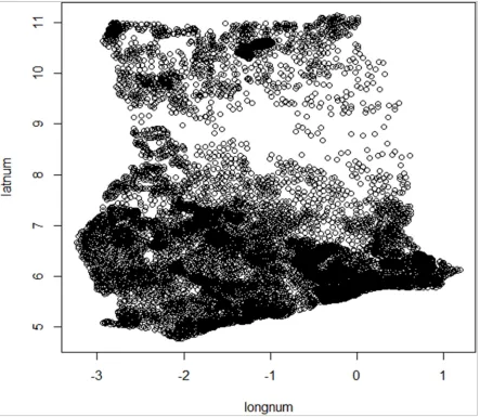
The dataset of the GLSS used to test performance of the models in this study consists of expenditure, economic and demographic histories corresponding to 16772 sampled households. Figure 1 and Table 1 respectively contain sample sites and the study variables.
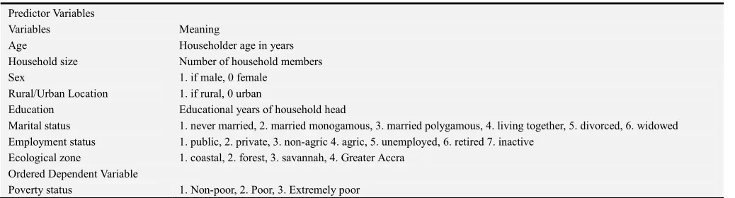
Table 1. Study Variables.
Predictor Variables
Variables Meaning
Age Householder age in years
Household size Number of household members
Sex 1. if male, 0 female
Rural/Urban Location 1. if rural, 0 urban
Education Educational years of household head
Marital status 1. never married, 2. married monogamous, 3. married polygamous, 4. living together, 5. divorced, 6. widowed Employment status 1. public, 2. private, 3. non-agric 4. agric, 5. unemployed, 6. retired 7. inactive
Ecological zone 1. coastal, 2. forest, 3. savannah, 4. Greater Accra Ordered Dependent Variable
Figure 1. Sample Sites of GLSS Data.
5. Results
A Spatial Cumulative Probit Model (SCPM) was fitted to the GLSS data in Ghana using Bayesian estimation discussed in Section 2.1 together with the simple aspatial CP model.
The purpose of data analysis in this section was to assess the effect of demographic and geo-socio-economic factors on poverty incidence and compare results of the SCPM and the aspatial CP model.
Using MCMC techniques in R [18], data was sampled from the full conditionals of parameters. Table 2 presents estimation results for posterior means and Bayesian Credible
Intervals (BCIs), at 5% level of significance, for the two models. The value 0 in the range of the BCI means that the variable is not significant.
The vector of 4 coefficients showed no significant difference in the point estimates between the two models, except in the thresholds (Table 2). The SCPM estimates of the thresholds are smaller than those from the CP model. Similarly, its standard errors are smaller than those of the CP model. These results confirm known international research about bias in aspatial estimates when using data that are spatially dependent [19].
Table 2. Parameter Estimates and P-values for Different OP Models.
Household Age
Model W XY (non-poor) XZ (poor) [Y \\]^_` [Z ab`
CP Model - 1.08 1.98 0.15 (0.14,0.17) 0.001 (-0.001,0.004)
SCPM 0.035 0.23 0.88 2.09 (0.45,3.14) 0.02 (-0.02,0.06)
Education Sex (Ref: c`dae`) Location (Ref: fghae)
Model [i jh] kl mn [o pae` [q rhsat
CP Model -0.06 (-0.07,-0.05) 0.05 (-0.05,0.14) -0.55 (-0.63,-0.48)
Employment Status (Ref: private)
Model [u (Public) [v (Inactive) [w (Sel no-ag) [x (Self agr) [Yy (unemp) [YY (Retired)
CP Model -0.22 (-0.38,-0.06) 0.19 (0.01,0.36) -0.17 (-0.29,-0.06) 0.18 (0.07,0.28) 0.02 (-0.20,0.24) -0.25 (-0.67,0.17) SCPM -2.92 (-5.92,-0.20) 2.54 (0.004,5.672) -2.32 (-4.48,-0.26) 2.40 (0.24,4.50) 0.24 (-3.14,3.70) -3.74 (-11.56,2.26)
Marital status (Ref: z^{|kb`|\)
Model [YZ }`{`h [Yi pktk [Yo Poly [Yq ~^nk•`n [Yu €^{kh•`n
CP Model 0.08 (-0.08,0.23) -0.14 (-0.24,-0.04) -0.50 (-0.73,-0.27) -0.008 (-0.18,-0.16) 0.06 (-0.09,0.20) SCPM 0.93 (-1.33,3.50) -1.87 (-3.82,-0.13) -6.70 (-11.72,-0.91) -0.05 (-2.65,2.61) 0.80 (-1.19,3.20)
Ecological zone (Ref: Coastal)
Model [Yv Greater Accra [Yw Forest [Yx Savannah
CP Model -0.30 (-0.47,-0.12) -0.05 (-0.15,0.04) 0.45 (0.35,0.55)
SCPM -3.91 (-7.30,-0.52) -0.76 (-2.39,-5.56) 5.88 (1.00,9.27)
In our application, statistically significant covariates were found to be strongly related to the outcome variable (Table 2). The coefficient of the variable household size (4-) for example, is statistically significant in both models; its contribution to change in the response being positive. This means that the economic conditions of households tended to deteriorate from non-poor to extremely poor for sites with higher household sizes. The positive relationship between poverty status and household size has been described by Ennin et al. [7] using logistic regression to estimate the probability of poverty based on the 2006 GLSS data. They reported that larger households negatively affected poverty levels in the country. Other international research on poverty, for example, Achia et al [11], Rusnak [12], and Dudek and Lisicka [6] came to similar conclusions regarding the negative effect of large household sizes on poverty.
Age of household head was found not to be statistically significant.
Education was found to reduce the risk of extreme poverty in both models; a one unit increase in number of years spent in school tended to decrease the risk of poor and extremely poor respectively. The negative association between education and extreme poverty has been described by Ennin et al. [7], and Tomori et al. [5]. Higher education may result in higher skills, better jobs, higher income and higher ability to purchase goods and services, which improves standard of living.
Extreme poverty was related to the residency of household heads in both models, with urbanites being at lower risk. This finding parallels the work of GSS [20] and Cook et al. [21], who respectively concluded that urban households continued to record lower average rate of poverty (10.6%) when compared to their rural counterparts (37.9%). Many other authors on the subject, for example Achia et al. [11], Ennim et al. [7], [6], and Dudek and Lisicka [22] concluded in their respective works that the incidence of poverty was higher in rural than in urban communities.
With ‘private employment’ as the reference category, the
impact of employment on poverty in this study is typical [5]; showing higher risk for the inactive and ‘Agric’ household heads in both models. Since the beta coefficients in both models were positive, being inactive or being employed in the agricultural sector, when compared to a privately employed household head, increases the chance of being in a severer poverty level. Retired workers saw an increased risk of non-poor but decreased risk of poor and extremely poor. With respect to the unemployed, there was an increased risk of extremely poor, even though that variable’s effect is not to be significant.
Whilst the Greater Accra and savannah ecological zone variables were statistically significant in both models, the contribution of the forest ecological zone variable was not significant in the CP model. The marginal effect of ecological zone shows that living in the savannah ecological zone, as opposed to the coastal ecological zone (being the reference category), decreased the risk of being in the non-poor category, but increased the risk of being in the non-poor and extremely poor categories respectively (Table 2). A similar and notable conclusion was reached in a study by Ennim et al. [7]. They identified households in the savannah ecological zone of Ghana to be almost four times poorer than those living in the coastal and forest zones. GSS [20] and Tomori et al. [5] in separate studies in Ghana and Albania respectively, also identified geographic divisions as a key determinant of poverty.
For this study, the savannah ecological zone, polygamous marriages and urban location were the most powerful predictors of poverty severity. Further details of the results of analysis are shown in Tables 2.
6. Spatial Prediction and Mapping
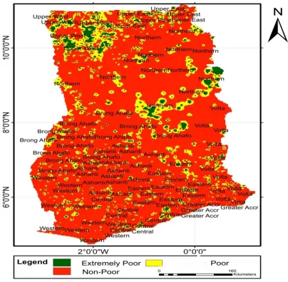
Figure 2. The SCPM’s Poverty Prediction Map for Ghana.
The prediction map (Figures 2) shows large regional differences in the distribution of household poverty, especially the ‘poor’ and ‘extremely poor’ categories. For instance, extreme poverty-risk was predicted to be especially higher in most of the northern half of the country. Within the forested middle belt and coastal zones, ‘non-poor’ dominated, showing the strong effect of spatial correlation, but also providing an empirical spatial character of poverty in Ghana. These findings conform to expert opinion on the subject. Generally, socio-econometricians [23, 24] and other authors [30, 21] agree that in a geographic environment, there can be a dominant, non-stochastic relationship between economic wellbeing and the agro-economic dynamics of a country. Several recent national and international reports point to similar dynamics of poverty in Ghana and in other parts of the world. Examples include reports by World Bank [25], International Fund for Agricultural Development (IFAD) [22], GSS [20], and Cook et al. [21].
To minimize or eliminate extreme poverty, stakeholder efforts should be directed towards areas with high posterior ranks. For example, extreme poverty incidence in the Upper West and some areas at the border between the Northern and
Brong Ahafo regions, extending eastwards, may be of concern to stakeholders. Conversely, stakeholders may wish to preserve areas with low incidence of extreme poverty, such as those shown in amber in Figure 2.
7. Conclusion
Generally, most applications in regional science rely heavily on data collected from different locations, and over large geographical areas. Models that can accurately describe such data, known as spatial data, are not well-developed, especially when the data are also categorical ordered.
The primary objective of this study was to develop a Bayesian classification model to improve the analysis and prediction of multi-categorical ordered data, especially when such data are collected over large geographical areas. The SCPM that ordered the population into three distinct categories (non-poor, poor, and extremely poor) was employed. Inference compared MCMC simulation results with the simple CP model.
packages. However, because the model does not incorporate spatial dependence in the estimation process, estimates were biased. This is a serious limitation for all non-spatial models when dealing with spatial data.
The SCPM model provides flexible ways to incorporate spatial dependence in the modelling framework, and thus, gave unbiased estimates of the parameters and their BCIs, whiles at the same time maintain the ordering of the data.
If policy interventions are intended to be effective at poverty reduction, then they should target the influence of the significant variables in this study.
References
[1] Nelder, J., Wedderburn R. W. M. (1972). Generalized linear models. J. Roy. Statist. Soc. Ser. A135: 370-384.
[2] Greene W. H., Hensher D. A., (2009). Modelling Ordered Choices. Cambridge: Cambridge University Press, 2010 xv, 365 p.: ill.; 25 cm. ISBN: 9780521194204.
[3] Agresti, A. (2007). An Introduction to Categorical Data Analysis. 2nd Ed., New York, John Wiley and Sons.
[4] Terza, J. (1985). Ordered Probit: A Generalization, Communications in Statistics -A. Theory and Methods, 14, pp. 1-11.
[5] Elena (Tomori), M., Zyka, E., Bici, R. (2014). Identifying Household Level Determinants of Poverty in Albania Using Logistic Regression Model (SSRN Scholarly Paper No. ID 2457441).
[6] Dudek, H., Lisicka, I. (2013). Determinants of poverty–binary logit model with interaction terms approach. Ekonometria, (3 (41), 65–77.
[7] Ennin C. C., Nyarko P. K., Agyeman A., Mettle F. O., Nortey E. N. N., (2011). Trend Analysis of Determinants of Poverty in Ghana: Logit Approach. Research Journal of Mathematics and Statistics 3 (1): 20-27, 2011, ISSN: 2040-7505.
[8] BARTOŠOVÁ, Jitka a Marie FORBELSKÁ (2013). Poverty Rate in Czech Households Depending on the Age, Sex and Educational Level. In LÖSTER, T. -- PAVELKA, T. International Days of Statistics and Economics. 7th ed. Slaný: Melandrium, 2013. s. 70-78, 9 s. ISBN 978-80-86175-87-4. [9] Saidatulakmal and Madiha Riaz (2012). Demographic
Analysis of Poverty, Rural-Urban Nexus. Research on Humanities and Social Sciences. Vol. 2, No. 6, 2012.
[10] Adebanji, A., Achia, T., Ngetich, R., Owino, J., Wangombe A. (2008). Spatial Durbin Model for Poverty Mapping and Analysis, European Journal of Social Sciences – Volume 5, Number 4.
[11] Thomas N. O., Achia, A. W., Nancy K. (2010). A Logistic
Regression Model to Identify Key Determinants of Poverty Using Demographic and Health Survey Data. European Journal of Social Sciences – Volume 13, Number 1 (2010). [12] Rusnak Z. (2012). Logistic regression model in poverty
analyses. ekonometria econometrics 1 (35)• 2012; issn 1507-3866.
[13] Williams, D. A. (1982). Extra-binomial variation in logistic linear models. Appl. Statist. 31: 144-148.
[14] Gelman A., Carlin J. B., Stern H. S., Dunson D. B., Vehtari A., Rubin D. B. (2014). Bayesian Data Analysis. Third Edition. CRC Press, Taylor and Francis Group, 6000 Broken Sound Parkway NW, Suite 300, Boca Raton, FL 33487-2742. [15] Neal, P. and Kypraios, T. (2015). Exact Bayesian inference via
data augmentation. 25: 333. https://doi.org/10.1007/s11222-013-9435-z, Springer US.
[16] Bayes (1763). An Essay towards solving a Problem in the Doctrine of Chances. By the late Rev. Mr. Bayes, communicated by Mr. Price, in a letter to John Canton, M. A. and F. R. S.
[17] De Oliveira, V. (2000). Bayesian prediction of clipped Gaussian random fields. Computational Statistics and Data Analysis, 34, 299–314.
[18] R Development Core Team, (2015). R: A Language and Environment for Statistical Computing. R Foundation for Statistical Computing, Vienna, Austria, ISBN 3-900051-07-0. http://www.R-project.org.
[19] Diggle PJ, Ribeiro PJ, Christensen OF (2003). An introduction to model-based geostatistics. In: Moller J, editor. Spatial statistics and computational methods Lecture notes in statistics. New York: Springer. 43–86.
[20] Ghana Statistical Service (GSS) (2014). Ghana Living Standards Survey Round 6 (GLSS6): Poverty Profile in Ghana (2005-2013), Main Report, Accra, Ghana.
[21] Cook E., Hague S., Mckay A. (2016). The Ghana Poverty and Inequality Report: Using the 6th Ghana Living Standards Survey. Accra, Ghana.
[22] The International Fund for Agricultural Development (2015). IFAD Annual Report 2014. International Fund for Agricultural Development Via Paolo di Dono, 44 - 00142 Rome, Italy.
[23] Jalan, J., Ravallion M. (1997). Spatial poverty traps? World Bank Policy Research Working Paper 1862.
[24] Bigman, D., Fofack, H. (2000). Geographical Targeting for Poverty Alleviation: An Introduction to the Special Issue. The World Bank Economic Review, VOL. 14, NO. li 129-45. [25] The World Bank (2015). Global Monitoring Report