Distributions Based on Record Values
Samah N. Sindi
Department of Statistics, Faculty of Science King Abdulaziz University, Jeddah, Saudi Arabia [email protected]
Gannat R. Al-Dayian
Department of Statistics, Faculty of Science King Abdulaziz University, Jeddah, Saudi Arabia [email protected]
Saman Hanif Shahbaz
Department of Statistics, Faculty of Science King Abdulaziz University, Jeddah, Saudi Arabia [email protected]
Abstract
The main objective of this paper is to suggest and study a new exponentiated general class (EGC) of distributions. Maximum likelihood, Bayesian and empirical Bayesian estimators of the parameter of the EGC of distributions based on lower record values are obtained. Furthermore, Bayesian prediction of future records is considered. Based on lower record values, the exponentiated Weibull distribution, its special cases of distributions and exponentiated Gompertz distribution are applied to the EGC of distributions.
Keywords: Lower record values, Maximum likelihood estimation, Bayesian estimation, empirical Bayesian estimation, Bayesian prediction.
1. Introduction
Bayesian prediction of record values has a special interest, as the best approach found until now, in many fields such as clinical trials, insurance, industry, architecture, physics, marketing, geography, and other fields. Recently, few studies are concerned with Bayesian prediction and both Bayesian and classical inferences for record values. Among others are Hsieh (2001), Ali-Mousa (2001,2003), Ali-Mousa et al. (2002), AL-Hussaini and Ahmed (2003a,b), Jaheen (2003), Madi and Raqab (2004), Ahmadi et al. (2005), Ahmadi and Doostparast (2006), Abdel-Aty et al. (2007), Al-Aboud and Soliman (2008), Ahmadi and MirMostafaee (2009).
non-Bayesian confidence intervals for the parameter in closed forms. Furthermore, he obtained a Bayesian prediction interval for the 𝑘𝑡ℎ future record in a closed form. For more details about exponentiated Weibull see (Nadarajah and Kotz (2006)).
Raqab and Ahsanullah (2001) derived exact expressions for the single and product moments of order statistics from the generalized exponential distribution. They used these moments to obtain estimators of the location and scale parameters of the model. Raqab (2002) derived exact expressions for means, variances and covariances of record values from the generalized exponential distribution. Jaheen (2004) derived Bayesian and empirical Bayesian estimators for the unknown parameter of the generalized exponential distribution based on record values. He obtained the estimates based on the squared error and the LINEX loss function. Furthermore, he obtained the prediction bounds for future lower record values by using both Bayesian and empirical Bayesian techniques. He, also, gave a numerical example to illustrate the results.
Ahmadi et al. (2009) studied the prediction of future k-record based on observed record which come from a general class of continuous distributions. They obtained the Bayes predictors of the sth future k-record under balanced type loss function. Nadar et al. (2012)
reviewed and derived some results on record values for some well known distributions and based on m records from Kumaraswamy's distribution. They also obtained the estimators of the parameters and for the future sth record value, when the m past record
values have been observed. They used the maximum likelihood and Bayesian approaches. Then, they illustrated the findings with actual and computer generated data.
Describing the layout of the paper; Section 2 is devoted to the construction of the new EGC of distributions. ML, Bayesian and empirical Bayesian estimators of a new introduced parameter are obtained. In addition, Bayesian prediction of future records, based on lower record values, is found. Section 3 deals with the application of all the mathematical work done in Section 2. The exponentiated Weibull distribution (Burr X)is considered in details. Furthermore, same special cases of the exponentiated Weibull distribution and other distributions are also been applied.
2. Exponentiated General Class
In this section the idea of the new EGC of distributions is displayed. ML, Bayesian and empirical Bayesian estimators based on lower record values are obtained. In addition, Bayesian predictions of future records are discussed.
AL-Hussaini and Ahmad (2003a) have introduced a general class denoted by (GC) of distributions. It includes the Weibull, compound Weibull, Pareto, beta, Gompertz and compound Gompertz among other distributions. The GC of distributions presents the populations with distribution function of the form
> 0, x, F(x)1exp[(x)] (1)
The idea of the construction of the new EGC of distributions is to raise the cdf of the GC, presented in relation (1), to the power θ, where θ is assumed to be a positive parameter. Thatis, the cdf of the EGC of distributions is expressed in the form
1 exp
, , 0.)
(x x x
F (2)
Thus, the density function is given by
1exp 1
exp
x x x
x
f , x, 0, (3)
where,
x
x, is a non-negative continuous function of xand γ. We assume that γ is a known parameter or (vector of parameters). That is, the unique unknown parameter of the EGC of distribution is θ. Where,
x, 0 as x0 and
x, as
x .
2.1 Estimation of the Parameter
This subsection concerns with the ML and Bayesian and empirical Bayesian estimation of the parameter θ of the EGC of distributions, based on lower record values. Furthermore, Bayesian prediction of future records is explained.
Suppose that 𝑚 lower record values, XL(1) x1,XL(2) x2,,XL(m) xm, are observed from the distribution with cdf and pdf given, respectively by (2) and (3). ML, Bayesian and empirical Bayesian estimators are obtained as follows.
2.1.1Maximum Likelihood Estimation
The likelihood function is given by (see Arnold et al. (1998))
𝐿(𝜃|𝑥)=𝑓(𝑥𝑚) ∏𝑚−1𝑖=0 𝑟(𝑥𝑖),
where, 𝑥 = (𝑥1, 𝑥2, … , 𝑥𝑚) and 𝑟(𝑥) = 𝑓(𝑥) 𝐹(𝑥), It follows that,
𝐿(𝜃|𝑥) =𝜃𝑚 𝑒𝑥𝑝(−𝜃𝜂(𝑥𝑚)) 𝑢(𝑥) , (4)
where,
𝑢(𝑥) = ∏ 𝜆′(𝑥
𝑖)𝑒−𝜆(𝑥𝑖)(1 − 𝑒−𝜆(𝑥𝑖)) −1
,
𝑚 𝑖=1
and
𝜂(𝑥𝑚) = −𝑙𝑛(1 − 𝑒−𝜆(𝑥𝑚)). (5)
Assuming that the parameter𝜃is unknown, the ML estimator (MLE) of 𝜃 is given by
𝜃̂𝑀𝐿 = 𝑚 𝜂(𝑥⁄ 𝑚), (6)
where, 𝜂(𝑥𝑚)is expressed in (5).
To study the properties of this estimator, the distribution of 𝜂(𝑥𝑚) is needed. The pdf of
𝑋𝑚 is given by
𝑓𝑋𝑚(𝑥) = 1
𝛤(𝑚)𝑓(𝑥)[−𝑙𝑛𝐹(𝑥)] 𝑚−1.
That is,
𝑓𝑋𝑚(𝑥) =
𝜃𝑚 𝛤(𝑚)𝜆
The pdf of 𝑍 = 𝑚 𝜂(𝑥 𝑚)
⁄ can be obtained by using simple transformation on (7) and is given as,
𝑓𝑍(𝑧) =(𝑚𝜃)𝑚
𝛤(𝑚) 𝑒
−𝜃𝑚 𝑧⁄ (1 𝑧)
𝑚+1
, >0 , (8)
which is the inverted gamma distribution with parameters (𝑚, 𝑚𝜃).
The expected value of 𝜃̂𝑀𝐿is
𝐸(𝜃̂𝑀𝐿) = 𝐸(𝑍) = 𝑚
𝑚−1𝜃. (9)
Therefore, the MLE of 𝜃 is a biased estimator and the unbiased estimator is
(𝑚 − 1) 𝜂(𝑥⁄ 𝑚). The variance of 𝜃̂𝑀𝐿 can be shown to be
𝑉𝑎𝑟(𝜃̂𝑀𝐿) = 𝑉𝑎𝑟(𝑍) =
𝑚2 (𝑚−1)2(𝑚−2)𝜃
2
(10)
2.1.2Bayesian Estimation
Under the assumption that the parameter 𝜃 is unknown, we can use the conjugate gamma prior with pdf
𝑔(𝜃) = 𝛽𝛿
𝛤(𝛿)𝜃
𝛿−1𝑒−𝛽𝜃 , 𝜃 > 0, (𝛽, 𝛿 > 0).
(11)
The posterior density function of 𝜃 given the data, denoted by 𝑞(𝜃|𝑥) is
𝑞(𝜃|𝑥) =[𝛽+𝜂(𝑥𝑚)]𝑚+𝛿
𝛤(𝑚+𝛿) 𝜃
𝑚+𝛿−1𝑒−𝜃[𝛽+𝜂(𝑥𝑚)]
.
(12)Under the squared error loss function, the Bayesian estimator of 𝜃 (denoted by 𝜃̂𝐵𝑆) is the mean of the posterior density and given by
.ˆ
0
BS
q x dTherefore,
𝜃̂𝐵𝑆 = 𝑚+𝛿
[𝛽+𝜂(𝑥𝑚)] . (13)
Under the LINEX loss function, the Bayes estimator of 𝜃 (denoted by 𝜃̂𝐵𝐿) is given by
𝜃̂𝐵𝐿 = − 1
𝑎𝑙𝑛 (𝐸(𝑒
−𝑎𝜃)). Hence,
𝜃̂𝐵𝐿 = 𝑚+𝛿
𝑎 𝑙𝑛 (1 + 𝑎
𝛽+𝜂(𝑥𝑚)), 𝑎 ≠ 0. (14)
2.1.3Empirical Bayesian Estimation
and the LINEX loss functions, respectively. For more details on the empirical Bayesian approach, see Maritz and Lwin (1989).
When the current (informative) sample is observed, suppose that 𝑛 past similar samples
𝑋𝑗,𝐿(1), 𝑋𝑗,𝐿(2), … , 𝑋𝑗,𝐿(𝑚) , 𝑗 = 1,2, … , 𝑛 are available with past realization 𝜃1, 𝜃2, … , 𝜃𝑛 of the random variable 𝜃. Each sample is assumed to be lower record sample of size 𝑚
obtained from the distribution with pdf given by (3). The likelihood function of the 𝑗𝑡ℎ
sample is given by (4) with 𝑥𝑚 being replaced by𝑥𝑗,𝑚. For a sample j, j = 1, 2,., n the MLE of the parameter 𝜃𝑗 can be rewritten by using (6).
𝜃̂𝑗 = 𝑍𝑗 = 𝑚 𝜂(𝑥⁄ 𝑗,𝑚). (15)
The conditional pdf of
𝑍
𝑗, j = 1,2,…, n, for a given 𝜃𝑗 is obtained from (8) in the form𝑓(𝑧𝑗|𝜃𝑗) = (𝑚𝜃𝑗)
𝑚
𝛤(𝑚) [ 1 𝑧𝑗]
𝑚+1
𝑒𝑥𝑝 − (𝑚𝜃𝑗⁄𝑧𝑗), 𝑧𝑗 > 0.
(16)
Which is the inverted gamma distribution with parameters (m, m𝜃𝑗). The marginal pdf of
𝑧𝑗 , 𝑗 = 1,2, … , 𝑛, is the compound distribution
𝑓𝑍𝑗(𝑧𝑗) = ∫ 𝑓(𝑧𝑗|𝜃𝑗) 𝑔(𝜃𝑗)
∞ 0
𝑑𝜃𝑗 ,
where f
zjj
and g
j are given by (16) and (11), respectively, after indexing θ in(11) by j. That is,
𝑓𝑍𝑗(𝑧𝑗) =
𝛽𝛿𝑚𝑚 𝐵(𝑚,𝛿)×
𝑧𝑗𝛿−1 (𝑚+𝛽𝑧𝑗)
𝑚+𝛿 , 𝑧𝑗 > 0. (17)
The method of moments estimators of the parameters 𝛽 and 𝛿 are given respectively by
𝛽̂ = 𝑚𝑠1
(𝑠2−𝑠12)(𝑚−1) and 𝛿̂ =
𝑠12
𝑠2−𝑠12. (18)
Then, the empirical Bayesian estimators of the parameter 𝜃 under the squared error and the LINEX loss functions are given, respectively, by
𝜃̂𝐸𝐵𝑆 = 𝑚+𝛿̂
𝛽̂+𝜂(𝑥𝑚), (19)
and
𝜃̂𝐸𝐵𝐿 = 𝑚+𝛿̂
𝑎 𝑙𝑛 (1 + 𝑎
𝛽̂+𝜂(𝑥𝑚)), 𝑎 ≠ 0, (20)
where, 𝛿̂ and 𝛽̂ are the estimators of 𝛽 and 𝛿 given by (18).
2.2 Bayesian Prediction of Future Records
Suppose that we have m lower records 𝑋𝐿(1) = 𝑥1, 𝑋𝐿(2) = 𝑥2, … , 𝑋𝐿(𝑚) = 𝑥𝑚 from the distribution with cdf and pdf given, respectively, by (2) and (3). Based on such a record sample, Bayesian prediction is needed for the 𝑠𝑡ℎ lower record, 1 < m < s. The conditional pdf of Y given the parameter 𝜃 is given by
𝑓(𝑦|𝜃) =[𝐻(𝑦)−𝐻(𝑥𝑚)]𝑠−𝑚−1
𝛤(𝑠−𝑚) × 𝑓(𝑦)
𝐹(𝑥𝑚) , 0 < y < 𝑥𝑚 < ∞, (21)
For the pdf of the EGC of distribution, f
y in (21) takes the form𝑓(𝑦|𝜃) =𝜃𝑠−𝑚𝜆′(𝑦)
𝛤(𝑠−𝑚) [𝑙𝑛 (
1−𝑒−𝜆(𝑥𝑚) 1−𝑒−𝜆(𝑦) )]
𝑠−𝑚−1
[1−𝑒−𝜆(𝑦)
1−𝑒−𝜆(𝑥𝑚)]
𝜃 𝑒−𝜆(𝑦)
1−𝑒−𝜆(𝑦), (22)
0 < y < 𝑥𝑚 < ∞.
The Bayes predictive density function of 𝑌 = 𝑋𝐿(𝑠) given the past m lower records is
𝑓∗(𝑦|𝑥) = ∫𝜃 𝑓(𝑦|𝜃) 𝑞(𝜃|𝑥) 𝑑𝜃, (23)
Where f
y and q
x are given by (22) and (12), respectively. Therefore, the result of the integral in (23) is𝑓∗(𝑦|𝑥) = 𝜆′(𝑦)
𝐵(𝑠−𝑚,𝑚+𝛿)[𝑙𝑛 (
1−𝑒−𝜆(𝑥𝑚) 1−𝑒−𝜆(𝑦))]
𝑠−𝑚−1 𝑒−𝜆(𝑦) 1−𝑒−𝜆(𝑦)
[𝛽+𝜂(𝑥𝑚)]𝑚+𝛿
[𝛽+𝜂(𝑦)]𝑠+𝛿 , 0 < 𝑦 < 𝑥𝑚 < ∞ (24)
Hence, the Bayesian prediction bounds 𝑌 = 𝑋𝐿(𝑠), are obtained by evaluating
𝑃(𝑌 ≥ 𝑡|𝑥), for some positive t. It follows, from (24) that
𝑃(𝑌 ≥ 𝑡|𝑥) = ∫𝑥𝑚𝑓∗
𝑡 (𝑦|𝑥) 𝑑𝑦. That is,
𝑃(𝑌 ≥ 𝑡|𝑥) = 1 − 1
𝐵(𝑚+𝛿,𝑠−𝑚)𝐼𝐵𝜀(𝑚 + 𝛿, 𝑠 − 𝑚). (25) And
𝜀 =𝛽+𝜂(𝑥𝑚)
𝛽+𝜂(𝑡) < 1.
For the special case, when s=m+1, which is practically of special interest. The Bayesian prediction for a future lower record value 𝑋𝑚+1can be obtained by using (25) as
𝑃(𝑋𝑚+1≥ 𝑡1|𝑥) = 1 − [𝛽+𝜂(𝑥𝑚)
𝛽+𝜂(𝑡1)]
𝑚+𝛿
. (26)
A 100 τ% Bayesian prediction interval for 𝑌 = 𝑋𝑚+1 is
𝑃[𝐿𝐿(𝑋) < 𝑌 < 𝑈𝐿(𝑋)] = 𝜏
,
where 𝐿𝐿(𝑋) and 𝑈𝐿(𝑋) are the lower and upper limits satisfying the following equations
𝑃(𝑌 > 𝐿𝐿(𝑋)|𝑥) = (1 + 𝜏) 2⁄ , (27)
and
𝑃(𝑌 > 𝑈𝐿(𝑋)|𝑥) = (1 − 𝜏) 2⁄ . (28)
It follows from (26), (27) and (5) that
𝜆 (𝐿𝐿(𝑋)) = −𝑙𝑛 {1 − 𝑒𝑥𝑝 [𝛽 − (𝛽 + 𝜂(𝑥𝑚)) ( 1−𝜏
2 )
−1 𝑚+𝛿⁄
]}. (29)
Similarly, from (26), (28) and (5), it can be shown that
𝜆 (𝑈𝐿(𝑋)) = −𝑙𝑛 {1 − 𝑒𝑥𝑝 [𝛽 − (𝛽 + 𝜂(𝑥𝑚)) (1+𝜏
2 )
−1 𝑚+𝛿⁄
3. Applications
In this section, we apply the exponentiated Weibull distribution to the classical Bayesian and empirical Bayesian estimation of the parameter 𝜃 of the EGC of distributions based on lower record values. In addition, Bayesian prediction of the future recordsis applied. However, the application of some special cases of the exponentiated Weibull distribution and the exponentiated Gompertz distribution are presented in Table 1 and Table 2.
3.1 Maximum Likelihood Estimation
The cdf and the pdf of a random variable having the exponentiated Weibull distribution are given, respectively, by
𝐹(𝑥) = [1 − exp (−(𝜇𝑥)𝛼)]𝜃, 𝑥 > 0 , 𝜇 > 0 , 𝛼 > 0 𝑎𝑛𝑑 𝜃 > 0 (31) and
𝑓(𝑥) = 𝜃𝛼𝜇𝛼𝑥𝛼−1𝑒−(𝜇𝑥)𝛼[1 − exp(−(𝜇𝑥)𝛼)]𝜃−1, 𝑥 > 0, 𝛼 > 0, 𝜇 > 0 𝑎𝑛𝑑 𝜃 > 0 (32) Where, 𝜃 𝑎𝑛𝑑 𝛼 are shape parameters and µ is a scale parameter.
Suppose that the lower record values, 𝑋𝐿(1) = 𝑥1, 𝑋𝐿(2) = 𝑥2, … , 𝑋𝐿(𝑚) = 𝑥𝑚, are from the exponentiated Weibulldistribution with cdf and pdf given respectively by (31), (32). Recall equation (2), one can see that (x)(x), (,), and (x)x1. The likelihood function is
𝐿(𝜃|𝑥) = (𝜃𝛼𝜇𝛼)𝑚𝑒𝜃𝑙𝑛(1−𝑒−(𝜇𝑥𝑚)𝛼)∏ 𝑒−(𝜇𝑥𝑖)𝛼 1−𝑒−(𝜇𝑥𝑖)𝛼 𝑚
𝑖=1 𝑥𝑖𝛼−1. (33)
Assuming that the parameter𝜃 is unknown, the MLE of 𝜃 is given by (6), which can be rewritten as
𝜃̂𝑀𝐿 = 𝑚
−𝑙𝑛(1−𝑒−(𝜇𝑥𝑚)𝛼). (34)
To study the properties of this estimate the distribution of 𝜂(𝑥𝑚) is needed. Applying equation (7) the pdf of 𝑋𝑚 is then given by
𝑓𝑥𝑚(𝑥) =𝜃𝑚𝛼𝜇𝛼
Γ(𝑚) 𝑥
𝛼−1𝑒−(𝑥𝜇)𝛼(1 − 𝑒−(𝜇𝑥)𝛼)𝜃−1(−𝑙𝑛(1 − 𝑒−(𝜇𝑥)𝛼))𝑚−1, x > 0. (35)
Hence, the pdf of 𝑍 = 𝑚 𝜂(𝑥 𝑚)
⁄ is given by (8).Which is the inverted gamma
distribution with parameters (𝑚, 𝑚𝜃). That is, the expected value and the variance of ˆ ML are given respectively, by (9) and (10).
3.2 Bayesian Estimation
Under the assumption that the parameter 𝜃 is unknown, we can use the conjugate gamma prior with pdf which is given by (11). The posterior density function of 𝜃 given the data, denoted by 𝑞(𝜃|𝑥), can be obtained by using (11) and (33) as
𝑞(𝜃|𝑥) =[𝛽−𝑙𝑛(1−𝑒−(𝜇𝑥𝑚)𝛼)]
𝑚+𝛿
𝛤(𝑚+𝛿) 𝜃
𝑚+𝛿−1𝑒−𝜃[𝛽−𝑙𝑛(1−𝑒−(𝜇𝑥𝑚)𝛼)]
Under a squared error loss function, the Bayesian estimator of 𝜃, 𝜃̂𝐵𝑆 is given by
𝜃̂𝐵𝑆 = 𝑚+𝛿
[𝛽−𝑙𝑛(1−𝑒−(𝜇𝑥𝑚)𝛼)]. (37)
Under the LINEX loss function, the Bayesian estimator of 𝜃, 𝜃̂𝐵𝐿 is given by
𝜃̂𝐵𝐿 = 𝑚+𝛿
𝑎 𝑙𝑛 (1 +
𝑎
𝛽−𝑙𝑛(1−𝑒−(𝜇𝑥𝑚)𝛼)), 𝑎 ≠ 0. (38) 3.3 Empirical Bayesian Estimation
When the prior parameters 𝛽 and 𝛿 are unknown, we may use the empirical Bayesian approach to get their estimates. Since the prior density (11) belongs to a parametric family with unknown parameters, such parameters are to be estimated using past samples. Applying these estimates in (37) and (38), we obtain the empirical Bayes estimate of the parameter 𝜃 based on the squared error and the LINEX loss functions, respectively.
When the current (informative) sample is observed, suppose that 𝑛 past similar samples
𝑋𝑗,𝐿(1), 𝑋𝑗,𝐿(2), … , 𝑋𝑗,𝐿(𝑚) , 𝑗 = 1,2, … , 𝑛 are available with past realization 𝜃1, 𝜃2, … , 𝜃𝑛of the random variable 𝜃. Each sample is assumed to be lower record sample of size 𝑚
obtained from the distribution with pdf given by (32). The likelihood function of the 𝑗𝑡ℎ
sample is given by (33) with 𝑥𝑚 being replaced by 𝑥𝑗,𝑚. For a sample j, j = 1, 2,…, n , the MLE of the parameter 𝜃𝑗 can be written by using (15) as
𝜃̂𝑗 = 𝑍𝑗 = 𝑚
−𝑙𝑛(1−𝑒−(𝜇𝑥𝑗,𝑚)
𝛼
)
. (39)
The conditional pdf of
𝑍
𝑗 , j = 1,2,…, n , for a given 𝜃𝑗 is given by (16).Which is the inverted gamma distribution with parameters (m , m𝜃𝑗). The marginal pdf of 𝑧𝑗 , 𝑗 = 1,2, … , 𝑛, is given by (17).Then, the empirical Bayesian estimates of the parameter 𝜃 under the squared error and the LINEX loss function are given by (19) and (20), respectively, as
𝜃̂𝐸𝐵𝑆 = 𝑚+𝛿̂
𝛽̂−𝑙𝑛(1−𝑒−(𝜇𝑥𝑚)𝛼), (40)
and
𝜃̂𝐸𝐵𝐿 = 𝑚+𝛿̂
𝑎 𝑙𝑛 (1 +
𝑎
𝛽̂−𝑙𝑛(1−𝑒−(𝜇𝑥𝑚)𝛼)), 𝑎 ≠ 0, (41) where, 𝛽̂ and 𝛿̂ are the moment estimates of 𝛽 and 𝛿 given by (18).
3.4 Bayesian Prediction of Future Records
Suppose that we have m lower records 𝑋𝐿(1) = 𝑥1, 𝑋𝐿(2) = 𝑥2, … , 𝑋𝐿(𝑚) = 𝑥𝑚 from the distribution with cdf and pdf are given respectively by (31) and (32). based on such a record sample, Bayesian prediction is needed for the 𝑠𝑡ℎ lower record, 1 < m < s. The conditional pdf of Y given the parameter 𝜃 is given by (22), it can be written as
𝑓(𝑦|𝜃) =𝜃𝑠−𝑚𝛼𝜇𝛼𝑦𝛼−1
Γ(𝑠−𝑚)
𝑒−(𝜇𝑦)𝛼 1−𝑒−(𝜇𝑦)𝛼[𝑙𝑛 (
1−𝑒−(𝜇𝑥𝑚)𝛼 1−𝑒−(𝜇𝑦)𝛼 )]
𝑠−𝑚−1
[1−𝑒−(𝜇𝑦)𝛼
1−𝑒−(𝜇𝑥𝑚)𝛼]
𝜃
The Bayes predictive density function of 𝑌 = 𝑋𝐿(𝑠) given the past m lower records is given by (24), it can be written in the form
𝑓∗(𝑦|𝑥) = 𝛼𝜇𝛼𝑦𝛼−1
Β(𝑠−𝑚,𝑚+𝛿)[𝑙𝑛 (
1−𝑒−(𝜇𝑥𝑚)𝛼
1−𝑒−(𝜇𝑦)𝛼 )]
𝑠−𝑚−1
𝑒−(𝜇𝑦)𝛼
1−𝑒−(𝜇𝑦)𝛼
[𝛽−𝑙𝑛(1−𝑒−(𝜇𝑥𝑚)𝛼)]𝑚+𝛿 [𝛽−𝑙𝑛(1−𝑒−(𝜇𝑦)𝛼)]𝑠+𝛿 ,
0 < y < 𝑥𝑚 < ∞. (43)
Bayesian prediction bounds 𝑌 = 𝑋𝐿(𝑠), are obtained by evaluating 𝑃(𝑌 ≥ 𝑡|𝑥), for some positive t. Which is given by (25).
For the special case, when s=m+1, which is practically of special interest. The Bayesian prediction for a future lower record value 𝑋𝑚+1can be obtained by using (26) as
𝑃(𝑋𝑚+1≥ 𝑡1|𝑥) = 1 − [𝛽−𝑙𝑛(1−𝑒−(𝜇𝑥𝑚)𝛼)
𝛽−𝑙𝑛(1−𝑒−(𝜇𝑡1)𝛼)] 𝑚+𝛿
. (44)
A 100 τ% Bayesian prediction interval for 𝑌 = 𝑋𝑚+1 is such that
𝑃[𝐿𝐿(𝑋) < 𝑌 < 𝑈𝐿(𝑋)] = 𝜏
,
where 𝐿𝐿(𝑋) and 𝑈𝐿(𝑋) are the lower and upper limits satisfying (27) and (28), it follows by using (29) that
𝐿𝐿(𝑋) = 1
𝜇{𝑙𝑛 {1 − 𝑒𝑥𝑝 [𝛽 − (𝛽 − 𝑙𝑛(1 − 𝑒
−(𝜇𝑥𝑚)𝛼)) (1−𝜏
2 ) −1
𝑚+𝛿 ⁄
]}
−1
}
1⁄𝛼
(45)
Similarly, from (30), one can find that
𝑈𝐿(𝑋) = 1
𝜇{𝑙𝑛 {1 − 𝑒𝑥𝑝 [𝛽 − (𝛽 − 𝑙𝑛(1 − 𝑒
−(𝜇𝑥𝑚)𝛼)) (1+𝜏
2 ) −1
𝑚+𝛿 ⁄
]}
−1
}
1 𝛼 ⁄
(46)
3.5 Special cases of the Exponentiated Weibull Distribution and the Exponentiated Gompertz Distribution
This subsection concerns with some special cases of the exponentiated Weibull distribution and the exponentiated Gompertz distribution. The ML, Bayesian and empirical Bayesian estimation, based on lower record values, of the parameter of each of the considered special cases and the exponentiated Gompertz distribution are obtained. In addition, Bayesian prediction of future records are found.
• Some special cases of the exponentiated Weibull distribution can be seen as follows:
1. When the parameters α and µ equal the value 1, the exponentiated Weibull distribution reduces to the generalized exponential distribution with density function
11 )
(x ex ex
2. When the parameter µ equals
2 1
and the parameter α is 2, the exponentiated
Weibull distribution reduces to the exponentiated Reyleigh with density function given by 1 2 1 2 1 2 2 2 1 ) (
x x
e e
x x
f ; x0, 0.
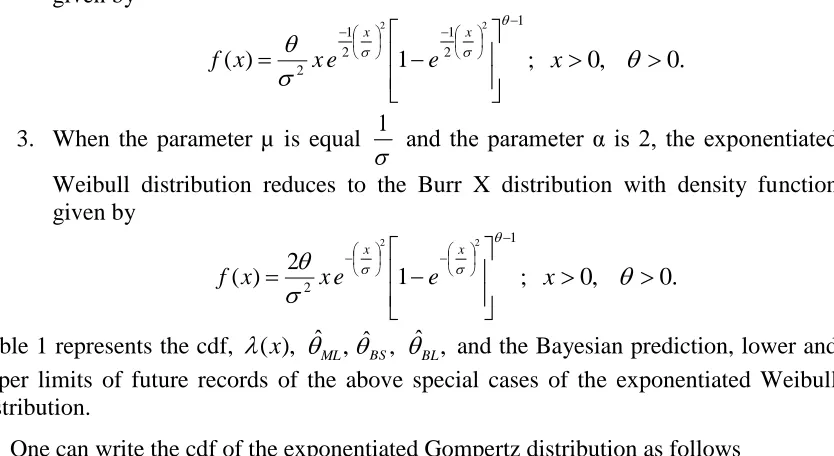
3. When the parameter µ is equal
1
and the parameter α is 2, the exponentiated
Weibull distribution reduces to the Burr X distribution with density function given by 1 2 2 2 1 2 ) (
x x
e e
x x
f ; x0, 0.
Table 1 represents the cdf, (x), ˆML,ˆBS, ˆBL, and the Bayesian prediction, lower and upper limits of future records of the above special cases of the exponentiated Weibull distribution.
• One can write the cdf of the exponentiated Gompertz distribution as follows
𝐹(𝑥) = (1 − 𝑒−𝑐(𝑒𝑎𝑥−1))𝜃; x0, a,c,0.
Since, the exponentiated Gompertz distribution is a member of the EGC of distributions, we write
1
)
( ax
e c x
.
The ML estimator of the parameter is
. 1 ln ˆ 1 ax
e c ML e m
However, the Bayesian estimators of the parameter under the squared error loss function and the LINEX loss function are given , respectively, by
, 1 ln ˆ 1 ax
e c BS e m
and
.
1
ln
1
ln
ˆ
1
ceaxBL
e
a
a
m
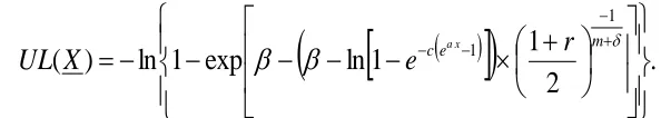
Finally, Bayesian prediction lower and upper limits of future records of the exponentiated Gompertz distribution are given by
,
2
1
1
ln
exp
1
ln
)
(
1 1
cer
me
X
and
.
2
1
1
ln
exp
1
ln
)
(
1 1
cer
me
X
UL
axThe results can be used to estimate parameters of other exponentiated distaributions that can be written as (2).
Table 1: Estimators and Bayesian prediction of the parameter of the special cases of the exponentiated Weibull distribution
Generalized exponential Exponentiated Reyleigh Burr X
Cdf
x
e x
F( ) 1 ( ) (1 )
2 2 1 x
e x
F ( ) (1 )
2
x
e x
F
) (x X 2 1 2 x 2 x ML ˆ
e xm
m
ln1
21 2
1 ln e xm
m
ln 1 exm 2m
BS
ˆ
e xm
m 1 ln
21 2
1 ln m x e m
2 1 ln m x e m BL ˆ
xm e a a m 1 ln 1 ln a m
21 2
1 ln 1
ln
xm
e a a m
2 1 ln 1 ln xm
e a Lower limit )) 1 ln( ( exp[ 1
ln{ exm
12 1m]}1
1m
2 1
exp[ 1 {ln{
122 2 1 } ))]} 1 ln(
( 1
m
x
e
1m
2 1 exp[ 1 {ln{
12 2
} ))]} 1
ln(
( 1
e xm
Upper limit )) 1 ln( ( exp[ 1
ln{ exm
12 1m]}1
1m
2 1
exp[ 1 {ln{
122 2 1 } ))]} 1 ln(
( 1
m
x e
1m
2 1
exp[ 1 {ln{
12
2
} ))]} 1
ln(
( 1
e xm
References
1. Abdel-Aty, Y., Franz, J., Mahmoud, M. A. W. (2007). Bayesian prediction based on generalized order statistics using multiply type-II censoring. Statistics, 41(6), 495-504.
3. Ahmadi, J., Doostparast, M. (2006). Bayesian estimation and prediction for some life distributions based on record values. Statist. Papers, 47(3), 373-392.
4. Ahmad, K. E., Fakhry, M. E. and Jaheen, Z. F. (1997). Empirical Bayes estimate and characterization of Burr X model. J. statist. Plann. Infer., 64, 297-308.
5. Ahmadi, J., MirMaostafaee, S. M. T. K. (2009). Prediction intervals for future records and order statistics coming from two parameter exponential distribution. Statist. Prob. Letters, 79, 977-983.
6. Ahmadi, J., Jozani, M. J., Marchand, E. and Parsian, A. (2009). Prediction of k-records from a general class of distributions under balanced type loss functions. Mertica, 70, 19-33.
7. Al-Aboud, F. M. and Soliman, A. A. (2008). Bayesian inference using record values from Rayleigh model with application. Euro. J. Opera. Res., 185, 659-672.
8. AL-Hussaini, E. K. and Ahmad A. A. (2003a). On Bayesian interval prediction of future record. Sociedad de Estadistica Investigation Operative 12, 79-99.
9. AL-Hussaini, E. K. and Ahmad, A. E. (2003b). On Bayesian predictive distributions of generalized order statistics. Metrika, 57, 165-176.
10. Ali-Mousa, M. A. M. (2001). Inference and prediction for Burr X based on records. Statistics, 35(4), 65-74.
11. Ali-Mousa, M. A. M. (2003). Bayesian prediction based on Pareto doubly censored data. Statistics, 37(1), 65-72.
12. Ali-Mousa, M. A. M, Jaheen, Z. F. and Ahmad, A. A. (2002). Bayesian estimation, prediction and characterization for the Gumbel model based on records. Statistics, 36(1), 65-74.
13. Arnold, B. C. and Balakrishnan N. and Nagarajah, H. N. (1998). Records, John Wiley and Sons, New York.
14. Gupta, R. D., Kundu, D. (1999). Generalized exponential distribution. Austr. NZJ. Statist. 41(2), 173-188.
15. Hsieh, P. H. (2001). On Bayesian predictive moments of next record values using three- parameter gamma priors. Commun. Statist.-Theory Meth., 30(4), 729-738.
16. Jaheen, Z. F. (1995). Bayesian approach to prediction with outliers from the Burr X model. Micro electron. Rel., 35, 45-47.
17. Jaheen, Z. F. (1996). Empirical Bayes estimation of the reliability and failure rate functions of the Burr X failure model. J. App. Statist. Sci., 3, 281-288.
18. Jaheen, Z. F. (2003). A Bayesian analysis of record statistics from the Gompertz model. Applied Mathematics and Computation. 145, 307-320.
19. Jaheen, Z. F. (2004). Empirical Bayes inference for generalized exponential distribution based on records. Commun. Statist.-Theory Meth., 33(8), 1851-1861.
21. Malinowska, I., Pawlas, P. and Szynal, D. (2006). Estimation of location and scale parameters for the BurrXII distribution using generalized order statistics. In Press, Available online at WWW. Sciencedirect.com.
22. Martiz, J. L., Lwin, T. (1989). Empirical Bayes Methods. 2nd ed. London:
Chapman and Hall.
23. Mudholkar, G. S., and Srivastava, D. K. (1993). Exponentiated Weibull family for analyzing bathtub failure data. IEEE Trans. Reliability, 42, 299-302.
24. Nadar, M., Papadopoulos, A. and Kizilaslan, F. (2012). Statistical analysis for Kumaraswamy's distribution based on record data. Stat Papers, doi: 10.1007/s00362-012-0432-7.
25. Nadarajah, S. and Kotz, S. (2006). The exponentiated type distributions. Acta. Appl. Math., 92, 97-111.
26. Raqab, M. Z. (2002). Inference for generalized exponential distribution based on record statistics. J. Statist. Plann. Inference, 104, 339-350.
27. Raqab, M. Z., Ahsanullah, M. (2001). Estimation of the location and scale parameters of generalized exponential distribution based on record statistics. J. Statist. Comput. Simul., 69(2), 109-124.
28. Sartawi, H. A. and Abu-Salih, M. S. (1991). Bayesian prediction bounds for the Burr X. Commun. Statist.-Theory Meth., 20(7), 2307-2330.