www.the-cryosphere.net/10/1799/2016/ doi:10.5194/tc-10-1799-2016
© Author(s) 2016. CC Attribution 3.0 License.
A simple equation for the melt elevation feedback of ice sheets
Anders Levermann1,2,3and Ricarda Winkelmann1,3
1Potsdam Institute for Climate Impact Research, Potsdam, Germany 2LDEO, Columbia University, NY, USA
3Institute of Physics, Potsdam University, Potsdam, Germany
Correspondence to:Anders Levermann ([email protected]) Received: 7 March 2016 – Published in The Cryosphere Discuss.: 12 April 2016 Revised: 15 July 2016 – Published: 18 August 2016
Abstract. In recent decades, the Greenland Ice Sheet has been losing mass and has thereby contributed to global sea-level rise. The rate of ice loss is highly relevant for coastal protection worldwide. The ice loss is likely to increase un-der future warming. Beyond a critical temperature thresh-old, a meltdown of the Greenland Ice Sheet is induced by the self-enforcing feedback between its lowering surface ele-vation and its increasing surface mass loss: the more ice that is lost, the lower the ice surface and the warmer the surface air temperature, which fosters further melting and ice loss. The computation of this rate so far relies on complex nu-merical models which are the appropriate tools for capturing the complexity of the problem. By contrast we aim here at gaining a conceptual understanding by deriving a purpose-fully simple equation for the self-enforcing feedback which is then used to estimate the melt time for different levels of warming using three observable characteristics of the ice sheet itself and its surroundings. The analysis is purely con-ceptual in nature. It is missing important processes like ice dynamics for it to be useful for applications to sea-level rise on centennial timescales, but if the volume loss is dominated by the feedback, the resulting logarithmic equation unifies existing numerical simulations and shows that the melt time depends strongly on the level of warming with a critical slow-down near the threshold: the median time to lose 10 % of the present-day ice volume varies between about 3500 years for a temperature level of 0.5◦C above the threshold and 500 years for 5◦C. Unless future observations show a signifi-cantly higher melting sensitivity than currently observed, a complete meltdown is unlikely within the next 2000 years without significant ice-dynamical contributions.
1 Introduction
In past decades global mean sea level has been rising, mainly by expansion of ocean waters and melting of ice on land (Church et al., 2013). Over the past 2 decades, the Greenland Ice Sheet has lost mass at an accelerating pace (Bamber et al., 2000; Box et al., 2012; van den Broeke et al., 2009; Fettweis et al., 2013; Mernild et al., 2011; Nick et al., 2009; Rignot et al., 2008, 2011; Shepherd and Wingham, 2007; Thomas et al., 2011). The ice loss is likely to increase under unabated greenhouse gas emissions (Clark et al., 2016; Fettweis et al., 2013; Goelzer et al., 2012; Graversen et al., 2011; Harper et al., 2012; Huybrechts et al., 2011; Levermann et al., 2013; Nowicki et al., 2013; Price et al., 2011).
rather a multi-millennial timescale is of relevance for coastal planning.
In this article we first recap the Vialov profile and add a simple representation of the melt elevation feedback towards a governing equation for a steady-state ice sheet in 1 dimen-sion, then we derive the critical warming threshold for the existence of an ice sheet in this simple model (Sect. 2). In Sect. 3 we derive a simple time evolution equation for the de-cay of the ice sheet after surface temperatures have exceeded the threshold. Finally we use observational estimates of the three characteristics that enter the model to estimate the de-cay time of the ice sheet under melting above the threshold (Sect. 4). Here solid ice discharge is neglected as well as any other ice sheet dynamics (Andresen et al., 2012; Howat and Eddy, 2012; Moon et al., 2012; Nick et al., 2009; Price et al., 2011; Straneo et al., 2011; Walsh et al., 2012). The framework that we introduce here can be used to include new physical processes that might be discovered in the future, e.g. potential changes in surface albedo through melting (Box et al., 2012) or aerosol-induced surface melt or the lack thereof (Polashenski et al., 2015).
2 Governing equation for shallow-ice steady states under melt elevation feedback
A non-linear threshold behaviour is generally associated with a fundamental self-enforcing feedback and thereby an as-sociated system memory (Levermann et al., 2012). For the Greenland Ice Sheet, such a feedback is given by the interac-tion between surface elevainterac-tion and surface melting (Weert-man, 1961). For illustration, we include this feedback in a well-established highly idealized ice profile of an ice sheet in 1 dimension, the so-called Vialov profile (Vialov, 1958). We introduce the melt elevation feedback in the simplest possi-ble way by assuming that the surface melt rate depends lin-early on the surface temperature and that the temperature de-creases linearly with the height of the ice surface following a constant atmospheric lapse rate.
2.1 Governing equation
We consider a highly simplified flow line model for an isothermal ice sheet grounded on a flat and rigid bed. The solution of the shallow-ice approximation in 1 dimension for the ice sheet elevation under these simplifying assumptions is the Vialov profile:
e
h(x)=hm
1−(x/L)(n+1)/nn/(2n+2), (1) wherehmis the maximum surface elevation andnis Glen’s flow law exponent (Glen, 1955).xdenotes the horizontal po-sition andLthe horizontal limit of the ice sheet. The inher-ent assumption of isothermal ice is a strong simplification, which needs to be kept in mind when interpreting the results.
The aim of this derivation is purposefully not a comprehen-sive representation of the ice flow but to derive a measure of the average height of the ice sheet and its dependence on changes in the surface mass balance. The surface mass bal-ance is considered to be spatially and temporally constant at a value,a, which will later be considered to be dependent on the surface elevation and thereby temporally variable. The overall horizontal extension of the ice sheet is set toL, and it is thereby assumed that any ice flow across this point is calved off into icebergs. This situation represents a confined ice-bearing bedrock topography as in most of Greenland’s interior (Howat et al., 2014). The mean surface elevation can then be computed to be
h=L−1 L
Z
0
dxh(x)=ω·hm. (2)
It is proportional to the maximum surface elevationhmwith a proportionality factor
ω≡
1
Z
0
dξ1−ξ(n+1)/nn/( 2n+2)
, (3)
which only depends on the flow law exponent.
The maximum surface elevation is determined by the sur-face mass balanceeaand the ice softnessAe:
hm=2(n−1)/(2n+2)·L1/2·
(n+2) ea
(ρg)n
e
A
1/(2n+2)
, (4)
with ρ being the ice density and g the gravity constant. We normalize all three quantities by definingh≡ω·hm/h0, a≡
ea/a0andA≡A/Ae 0, wherea0is the accumulation rate
on the ground, i.e. in the absence of an ice sheet, and A0=a0/ (ρg)n(·L)(n+1)
with=h0/L being the typ-ical height-to-width ratio.h0is the equilibrium line altitude of the considered ice sheet in the initial equilibrium situa-tion. Values fora0,h0andLare later chosen to resemble the conditions of the Greenland Ice Sheet.
The non-dimensional surface elevation,h, of the ice sheet can then be expressed as
h=a
A
1/m
. (5)
For the Vialov profile, m=2(n+1) where the Glen flow law exponent is commonly chosen to be aroundn=3, which yieldsm=8.
We introduce the melt elevation feedback in its simplest form through a dependency of the surface melt rate on the surface elevation:
a=a0+γ 0·h, (6)
0 Tc
0 hc
Ice thickness
Ground temperature
Unstable
Stable
Stable
hm - γ · Г · h + ∆T = 0
Figure 1.Ice sheet hysteresis. If the ice sheet is in an unstable con-figuration (dashed black branch), a slight perturbation will either cause it to converge into the stable state (upper red branch) or to melt completely. For a given temperature, the dotted line gives the critical surface elevation (Sect. 3). If the surface elevation is lower
thanhc, a complete meltdown of the ice sheet is inevitable. Once
the temperature threshold,Tc, is crossed, the time for a collapse of
a certain fraction of the ice sheet can be estimated via Eq. (17).
rate per degree of warming, which is regularly measured and comprises a large number of physical processes (e.g. Box, 2013). For simplicity we rescale the surface mass balance by the constant ice softness parameter, A, to obtainh=(a0+ γ 0·h)1/m. The steady-state solution for the surface elevation of the ice sheet is thus governed by the following equation:
hm−γ 0·h−a0=0, (7)
which has two positive solutions forhas long as the surface mass balance on the ground is negative, i.e.a0<0. Note that the surface mass balance can be positive even ifa0<0. If the ice sheet is in an unstable configuration, a slight perturbation will either cause it to converge into the stable state with a positive surface mass balance or to melt completely.
Our simple approach qualitatively captures the basic hys-teresis behaviour of the Greenland Ice Sheet caused by the melt elevation feedback (Fig. 1, in which we have assumed the surface mass balance to depend linearly on temperature): For a given surface temperature, a stable state of the ice sheet (red line) annihilates an external perturbation in surface el-evation by changes in surface mass balance (grey arrows). The unstable solution branch defines the basin of attraction for the stable state. A surface elevation that is lower than the unstable solution branch cannot be sustained. In that case the melting reduces the surface elevation to practically zero even without further external perturbation (grey arrows). Beyond a certain surface temperature threshold (vertical dotted line), no ice sheet can be sustained.
2.2 Critical surface mass balance in steady state
As illustrated in Fig. 1, there is a critical temperature above which the ice sheet is not sustainable. Let us denote the cor-responding surface elevation byhc. The critical point(Tc, hc)
has to fulfill two conditions, i.e. being a solution of the gov-erning Eq. (7) and minimum of the function
F (h)=hm−γ 0·h−a0, (8)
which we can determine by setting the derivative of F to zero. Consequently,
hc=
0·γ m
1/(m−1)
. (9)
Inserting this into the governing equation yields the critical surface mass balance at the ground:
a0c= −(m−1)·
0·γ
m
m/(m−1)
. (10)
For illustrative purposes we have assumeda0 to decline linearly with the surrounding temperature and plotted the so-lution of Eq. (7) against that temperature with an arbitrary offset in Fig. 1.
3 A simple temporal equation for the melt elevation feedback
Once the critical surface mass balance and surface elevation threshold (as derived in the previous Sect. 2) is transgressed, a meltdown of the ice sheet is inevitable in our conceptual model. Let us define the timeτα as the time it takes to melt a fractionαof the initial ice volume and the threshold tem-peratureTcas the temperature above the pre-industrial level at which the surface mass balance becomes negative. Robin-son et al. (2012) find a range of 0.8–3.2◦C for the thresh-old warming beyond which no ice sheet can be sustained on Greenland. Their best estimate for the threshold is 1.6◦C above pre-industrial level. The study uses a regional climate model of intermediate complexity (Robinson et al., 2010) coupled to the SICOPOLIS (SImulation COde for POLyther-mal Ice Sheets) ice sheet model (Greve, 1997). Using a dif-ferent model combination, Ridley et al. (2010) find that in their model the ice sheet cannot be sustained for a warm-ing of 2◦C. They combine the HadCM3 atmosphere–ocean general circulation model (Gordon et al., 2000) with an at-mospheric resolution of 2.5◦×3.75◦(Pope et al., 2000) to an ice sheet model of 20 km horizontal resolution (Huybrechts and De Wolde, 1999).
0
2
4
6
Warming above threshold [
◦C]
1
3
5
Time to lose 10% of ice [ka]
Ridley et al. (2010)
Robinson et al. (2012)
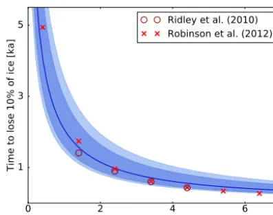
Figure 2.Decay time of the Greenland Ice Sheet. The decay time depends critically on the level of warming above the temperature threshold. Shown are the median (black line), likely (18–83 % quan-tiles, dark blue shading) and very likely (5–95 % quanquan-tiles, light blue shading) ranges for the time to melt 10 % of the present-day ice volume, estimated via Eq. (17). The red circles and crosses in-dicate the results from process-based model simulations by Ridley et al. (2010) and Robinson et al. (2012) respectively.
percentage ice volume change, a constant horizontal ice sur-face area was assumed which renders the analysis concep-tual in nature. Thus the quantitative interpretation of the melt times are subject to this additional simplification.
For a fixed anomalous melt rate 1a0= −γ·1T in re-sponse to an anomalous temperature increase1T =T −Tc above this threshold temperature,Tc, the decay time without any feedbacks would be
τ0= − h0 1a0
= h0
γ·1T. (11)
Since the surface temperature increases with decreasing ele-vation, this zero-order estimate for the decay time is higher than the actual value. As a first-order correction to the situa-tion of fixed melting, let us assume that the anomalous sur-face mass balance behaves as
1a=1a0+ 1 τγ
·(h−h0), (12)
whereτγ =1/(γ·0). From the relation dh/dt=1a, we then obtain
d1h
dt = −1a0+ 1h
τγ
, (13)
if 1h≡h0−h is defined as the reduction in height. For a time-dependent melting induced by surface warming1a0=
−γ·1T, the general solution of Eq. (13) is
1h(t )=γ·
t
Z
0
dt01T (t0)·e(t−t0)/τγ. (14)
This equation corresponds to a linear response theory with the melting−γ·1T as forcing and an exponential response function
R(t0)=et0/τγ. (15)
Linear response theory states that the convolution of Eq. (14) yields the linear response of the system (Good et al., 2011; Winkelmann and Levermann, 2013). Note that linear re-sponse theory is generally used as an approximation of a non-linear system to relatively weak forcing. In these cir-cumstances the response function has to decline with time because it represents the history of the system’s response to past perturbation. For example, if the response function was a declining exponentialR(t0)=e−t0, this would mean that the effect of forcing that occurred in the past, i.e. prior to the timetthat is considered, becomes exponentially less relevant for the current system response. Here, however, the response function isincreasing with time, which means that the past deviation from the steady state is amplified as expected near an unstable fixed point. The exponent 1/τγ can be considered the Lyaponov exponent of the system.
Given the boundary condition 1h(t=0)=0 for a con-stant temperature increase1T, Eq. (14) becomes
1h(t )=h0·
τ
γ τ0
−τγ
τ0
·et /τγ
−h0
τ0
−h0
τγ
. (16)
The decay time for a relative volume reduction ofαis then given by
τα= 1 γ 0·log
1+α·0·h0
1T
, (17)
where log denotes the natural logarithm. Equation (17) is de-noted the decay time equation hereafter.
4 Estimating the melt time of the Greenland Ice Sheet from observables
In this simplified approach, the collapse time is thus a func-tion of three observable quantities: the equilibrium line alti-tude,h0, the atmospheric lapse rate,0, and the melting sen-sitivity to temperature,γ. The average equilibrium line alti-tude of the Greenland Ice Sheet is at about 1150 m (Box and Steffen, 2001). The observed range for the atmospheric lapse rate is estimated to be between 5±2◦C km−1(Fausto et al., 2009; Gardner and Sharp, 2009) and current estimates for the melting sensitivity scatter around 4.4±2 cm year−1◦C−1 (Box, 2013). In order to obtain an estimate of the decay time and the uncertainty around this estimate we use Eq. (17) and choose the lapse rate and melting sensitivity uniformly ran-domly from these observed intervals (Table 1, Figs. 2–4).
Table 1.Decay time. Time period after which different percentages of volume loss have occurred at different warming levels. Provided are the median values of the distributions from Figs. 2 and 3 together with the lower and upper limits that are derived respectively from the upper and lower limits of the uncertainty range of the observed melting sensitivity and atmospheric lapse rate. The simple decay time equation (Eq. 17) does not take any ice dynamic effects into account and its translation to ice volume assumes a constant horizontal ice sheet area. Thus the values provided here best fit the complex model simulations only when these assumptions are reasonably well justified, which is most likely not the case for high ice loss such as 50 or 100 % of the original ice volume.
Volume loss 0.5◦C 1◦C 2◦C 3◦C 4◦C 5◦C
10 % Lower 2140 years 1320 years 760 years 530 years 410 years 330 years
Median 3430 years 2040 years 1140 years 790 years 610 years 500 years
Upper 7290 years 4120 years 2210 years 1520 years 1150 years 930 years
50 % Lower 4920 years 3600 years 2460 years 1900 years 1550 years 1320 years
Median 8740 years 6170 years 4040 years 3040 years 2450 years 2090 years
Upper 20 740 years 13 920 years 8640 years 6310 years 4980 years 4120 years
100 % Lower 6340 years 4920 years 3600 years 2910 years 2460 years 2140 years
Median 11 610 years 8730 years 6160 years 4840 years 4020 years 3500 years
Upper 28 710 years 20 740 years 13 920 years 10 630 years 8640 years 7290 years
the melt time of the Greenland Ice Sheet, assuming uniform probability distributions for both0andγ within the above intervals. Figure 2 shows the histograms of the time until 10 % of its present-day ice volume (corresponding to 0.7 m global sea-level rise) is melted for different warming scenar-ios. The melt time strongly depends on the level of warming beyond the temperature threshold: the median estimate varies from more than 2000 years for a warming of+1◦C to less than 500 years for a warming of+5◦C.
Existing numerical simulations of a decay of the Green-land Ice Sheet (Ridley et al., 2010; Robinson et al., 2012) differ in their trajectories for the total ice volume, but exhibit a characteristic functional form when the relative ice volume is expressed as a function of the temperature anomaly above the critical temperature threshold (Fig. 2). This characteristic relation is captured by our first-order equation for the de-cay time, embedding the results from process-based models into a simple analytical framework. This approach provides a good approximation if, on the one hand, the volume loss is large enough for the melt elevation feedback to become rel-evant and, on the other hand, the melting dominates the ice loss in contrast to the dynamic ice discharge.
Since the simple equation provided here does not account for any dynamic discharge or even ice motion, the results from Eq. (17) strongly deviate from numerical simulations when the ice has time to adjust dynamically to the volume loss. This can be seen for a stronger ice loss of 50 % of the initial volume where the functional dependence between the decay time and the temperature anomaly clearly follows a different functional form than predicted by Eq. (17)(Fig. 3).
Since the melt time is a monotonically decreasing func-tion of both the lapse rate and the melting sensitivity, the upper and lower limits of the estimates can be directly com-puted from the observed uncertainty interval of these quan-tities. However, the functional form of Eq. (17) introduces a
0 2 4 6
Warming above threshold [◦C]
5 10 15 20
Time to lose 50% of ice [ka]
Robinson et al. (2012)
Figure 3.Time until 50 % of the Greenland Ice Sheet is melted. Shown are the median (black line) and the likely (18–83 % per-centiles, dark blue shading) and very likely (5–95 % perper-centiles, light blue shading) ranges for the time to melt 50 % of the
present-day ice volume, estimated via the equation for the decay timeτα.
The red crosses indicate the results from process-based model sim-ulations by Robinson et al. (2012).
specific structure into the histogram of the melt time which is highly skewed towards the low end (Table 1 and Fig. 4). For increasing warming levels the histogram shifts towards lower decay times. At the same time the histogram narrows and higher decay times become less frequent within the cho-sen parameter range (see description above).
5 Discussion and conclusion
P
ro
b
a
b
ili
ty
d
e
n
s
it
y
#
#
#
#
(a)
(b)
(c)
(d)
Median Likely range Very likely range
P
ro
b
a
b
ili
ty
d
e
n
s
it
y
P
ro
b
a
b
ili
ty
d
e
n
s
it
y
P
ro
b
a
b
ili
ty
d
e
n
s
it
y
Time to lose 10 % of ice [years]
Figure 4.Likelihood for 10 % decay of Greenland Ice Sheet. Shown are the probabilities for the ice sheet to lose 10 % of its initial ice
volume in a certain time period for surface warming of(a)+1◦C,
(b)+2◦C,(c)+3◦C and(d)+4◦C above the threshold. The
me-dian is indicated by the black line, and the likely and very likely ranges are shaded in dark and light blue respectively.
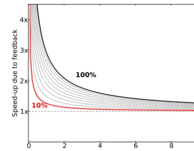
ing warming above the threshold (Eq. 17). The simple equa-tion of the decay time quantitatively reproduces the range given by simulations with process-based models. The rela-tive speed-up of ice loss due to the melt elevation feedback (Fig. 5) is estimated, using the central values of the param-eter ranges, i.e. equilibrium line altitude h0=1150 m,
at-0 2 4 6 8 10
Warming above threshold [◦C]
1x 2x 3x 4x
Speed-up due to feedback
10 %
100 %
Figure 5.Role of melt elevation feedback in melting of Greenland Ice Sheet declines with increasing temperature. Shown is the ratio of melt time with melt elevation feedback over melt time without the
feedbackτα/τ0. Each line represents the ratio for a loss of different
percent of the initial ice volume. The red line shows the ratio of the decay time with feedback over the decay time without feedback for a 10 % ice loss (corresponding to Figs. 2 and 4). The influence of the feedback becomes less dominant with stronger warming above the
critical threshold (xaxis). Near the threshold the melt time without
feedback diverges stronger (1/1T) than the melt time with
feed-back which declines logarithmically.
mospheric lapse rate0=5◦C km−1and melting sensitivity γ=4.4 cm year−1◦C−1. The feedback becomes more dom-inant near the threshold compared to larger temperature in-creases for which the external climatic forcing is more rele-vant.
The simple equation provided here is clearly limited in its applicability. The role of the ice material properties is com-prised into one parameter, the melting sensitivity of the ice to a temperature increase at the surface. This sensitivity will in general vary not only with time but also spatially and due to the melting itself. Similarly, the feedback role of the sur-rounding climate is represented by only one parameter, the atmospheric lapse rate which will again vary spatially but also with time as the ice surface declines.
caused by surface melting and dynamic discharge is limited by margin thinning and retreat.
Some studies suggest (Graversen et al., 2010; Price et al., 2011) that the dynamic discharge from Greenland is strongly limited by the ice sheet’s bottom topography, for which esti-mates yield an upper bound of approximately 5–13 cm dur-ing the next century. Over a period durdur-ing which the ice loss is dominated by the feedback and the ice-dynamic effect is limited, our approach provides a quantitative estimate of the melt time based on observable quantities. Equation (17) can thus be used if new observations suggest an altered melting sensitivity or changes in the atmospheric response to Green-land ice loss.
For a temperature increase of 5◦C, which could be reached within this century (IPCC, 2013), the median rate of sea-level contribution is about 1.4 mm year−1, which is about 4 times that of its current contribution of about 0.4 mm year−1 (Rig-not et al., 2011; Shepherd et al., 2012). Even for extremely high temperatures, however, the Greenland Ice Sheet cannot melt infinitely fast – our results show that a complete disinte-gration within the next 2 millennia is highly unlikely unless ice dynamics effects become dominant or the melting sen-sitivity is significantly higher than currently observed. For a global mean temperature increase below 2◦C, as agreed upon during the 2015 Paris UNFCCC climate summit, the threshold temperature would only be exceeded mildly and the decay time of the Greenland Ice Sheet would be multi-millennial.
Acknowledgements. The research leading to these results received funding from the European Union Seventh Framework Programme FP7/2007-2013 under Grant Agreement no. 603864.
Edited by: X. Fettweis
Reviewed by: two anonymous referees
References
Allen, M. R., Frame, D. J., Huntingford, C., Jones, C. D., Lowe, J. A., Meinshausen, M., and Meinshausen, N.: Warming caused by cumulative carbon emissions towards the trillionth tonne, Nature, 458, 1163–1166, doi:10.1038/nature08019, 2009.
Andresen, C. S., Straneo, F., Ribergaard, M. H., Bjørk, A. A., An-dersen, T. J., Kuijpers, A., Nørgaard-PeAn-dersen, N., Kjær, K. H., Schjøth, F., Weckström, K., and Ahlstrøm, A. P.: Rapid response of Helheim Glacier in Greenland to climate variability over the past century, Nat. Geosci., 5, 37–41, doi:10.1038/ngeo1349, 2012.
Bamber, J. L., Hardy, R. J., and Joughin, I.: An analysis of balance velocities over the Green land ice sheet and comparison with synthetic aperture radar interferometry, J. Glaciol., 46, 67–74, doi:10.3189/172756500781833412, 2000.
Box, J. E.: Greenland ice sheet mass balance reconstruction, Part II: Surface mass balance (1840–2010), J. Climate, 26, 6974–6989, doi:10.1175/JCLI-D-12-00518.1, 2013.
Box, J. E. and Steffen, K.: Sublimation on the Greenland Ice Sheet from automated weather station observations, J. Geophys. Res.-Atmos., 106, 33965–33981, 2001.
Box, J. E., Fettweis, X., Stroeve, J. C., Tedesco, M., Hall, D. K., and Steffen, K.: Greenland ice sheet albedo feedback: thermo-dynamics and atmospheric drivers, The Cryosphere, 6, 821–839, doi:10.5194/tc-6-821-2012, 2012.
Charbit, S., Paillard, D., and Ramstein, G.: Amount of CO2
emis-sions irreversibly leading to the total melting of Greenland, Geo-phys. Res. Lett., 35, 1–5, doi:10.1029/2008GL033472, 2008. Church, J. A., Clark, P. U., Cazenave, A., Gregory, J. M., Jevrejeva,
S., Levermann, A., Merrifield, M. A., Milne, G. A., Nerem, R. S., Nunn, P. D., Payne, A. J., Pfeffer, W. T., Stammer, D., Un-nikrishnan, A. S.: Sea Level Change, Chapter 13, in: Climate Change 2013 – The Physical Science Basis, Working Group I Contribution to the Fifth Assessment Report of the Intergovern-mental Panel on Climate Change, Cambridge University Press, doi:10.1017/CBO9781107415324.026, 2013.
Clark, P. U., Shakun, J. D., Marcott, S. A., Mix, A. C., Eby, M., Kulp, S., Levermann, A., Milne, G. A., Pfister, P. L., Santer, B. D., Schrag, D. P., Solomon, S., Stocker, T. F., Strauss, B. H., Weaver, A. J., Winkelmann, R., Archer, D., Bard, E., Gold-ner, A., Lambeck, K., Pierrehumbert, R. T., and PlattGold-ner, G.-K.: Consequences of 21st Century Policy for Multi-Millennial Cli-mate and Sea-Level Change, Nat. Clim. Chang., 6, 360–369, doi:10.1038/NCLIMATE2923, 2016.
Fausto, R. S., Ahlstrøm, A. P., Van As, D., Bøggild, C. E., and Johnsen, S. J.: A new present-day temperature parameterization for Greenland, J. Glaciol., 55, 95–105, doi:10.3189/002214309788608985, 2009.
Fettweis, X., Franco, B., Tedesco, M., van Angelen, J. H., Lenaerts, J. T. M., van den Broeke, M. R., and Gallée, H.: Estimating the Greenland ice sheet surface mass balance contribution to fu-ture sea level rise using the regional atmospheric climate model MAR, The Cryosphere, 7, 469–489, doi:10.5194/tc-7-469-2013, 2013.
Fürst, J. J., Goelzer, H., and Huybrechts, P.: Ice-dynamic pro-jections of the Greenland ice sheet in response to atmo-spheric and oceanic warming, The Cryosphere, 9, 1039–1062, doi:10.5194/tc-9-1039-2015, 2015.
Gardner, A. S. and Sharp, M.: Sensitivity of net mass-balance es-timates to near-surface temperature lapse rates when employing the degree-day method to estimate glacier melt, Ann. Glaciol., 50, 80–86, doi:10.3189/172756409787769663, 2009.
Glen, J. W.: The Creep of Polycrystalline Ice, P. Roy. Soc. A-Math. Phy., 228, 519–538, 1955.
Goelzer, H., Huybrechts, P., Raper, S. C. B., Loutre, M.-F., Goosse, H. and Fichefet, T.: Millennial total sea-level commitments pro-jected with the Earth system model of intermediate complexity LOVECLIM, Environ. Res. Lett., 7, 045401, doi:10.1088/1748-9326/7/4/045401, 2012.
Goelzer, H., Huybrechts, P., Fürst, J. J., Nick, F. M., Andersen, M. L., Edwards, T. L., Fettweis, X., Payne, A. J., and Shannon, S.: Sensitivity of Greenland ice sheet projections to model formu-lations, J. Glaciol., 59, 733–749, doi:10.3189/2013JoG12J182, 2013.
Gordon, C., Cooper, C., Senior, C. A., Banks, H., Gregory, J. M., Johns, T. C., Mitchell, J. F. B., and Wood, R. A.: The simulation of SST, sea ice extents and ocean heat transports in a version of the Hadley Centre coupled model without flux adjustments, Clim. Dynam., 16, 147–168, doi:10.1007/s003820050010, 2000. Graversen, R. G., Drijfhout, S., Hazeleger, W., Wal, R., Bintanja, R., and Helsen, M.: Greenland’s contribution to global sea-level rise by the end of the 21st century, Clim. Dynam., 37, 1427–1442, doi:10.1007/s00382-010-0918-8, 2010.
Graversen, R. G., Drijfhout, S., Hazeleger, W., van de Wal, R., Bin-tanja, R., and Helsen, M.: Greenland’s contribution to global sea-level rise by the end of the 21st century, Clim. Dynam., 37, 1427– 1442, doi:10.1007/s00382-010-0918-8, 2011.
Gregory, J. M., Huybrechts, P., and Raper, S. C. B.: Threat-ened loss of the Greenland ice-sheet, Nature, 428, 616, doi:10.1038/428616a, 2004a.
Gregory, J. M., Huybrechts, P., and Raper, S. C. B.: Threat-ened loss of the Greenland ice-sheet, Nature, 428, 2513–2513, doi:10.1038/nature02512, 2004b.
Greve, R.: Application of a polythermal three-dimensional ice sheet model to the Greenland Ice Sheet: Response to steady-state and transient climate scenarios, J. Climate, 10, 901–918, doi:10.1175/1520-0442(1997)010<0901:AOAPTD>2.0.CO;2, 1997.
Greve, R.: On the response of the Greenland ice sheet to greenhouse climate change, Climate Change, 46, 289–303, 2000.
Harper, J., Humphrey, N., Pfeffer, W. T., Brown, J., and Fet-tweis, X.: Greenland ice-sheet contribution to sea-level rise buffered by meltwater storage in firn, Nature, 491, 240–243, doi:10.1038/nature11566, 2012.
Howat, I. M. and Eddy, A.: Multi-decadal retreat of Greenland’s marine-terminating glaciers, J. Glaciol., 57, 389–396, 2012. Howat, I. M., Negrete, A., and Smith, B. E.: The Greenland Ice
Mapping Project (GIMP) land classification and surface eleva-tion data sets, The Cryosphere, 8, 1509–1518, doi:10.5194/tc-8-1509-2014, 2014.
Hurkmans, R. T. W. L., Bamber, J. L., Davis, C. H., Joughin, I. R., Khvorostovsky, K. S., Smith, B. S., and Schoen, N.: Time-evolving mass loss of the Greenland Ice Sheet from satellite al-timetry, The Cryosphere, 8, 1725–1740, doi:10.5194/tc-8-1725-2014, 2014.
Huybrechts, P. and De Wolde, J.: The Dynamic Response of the Greenland and Antarctic Ice Sheets to Multiple-Century Climatic warming, J. Climate, 12, 2169–2188, 1999.
Huybrechts, P., Goelzer, H., Janssens, I., Driesschaert, E., Fichefet, T., Goosse, H., and Loutre, M. F.: Response of the Greenland and Antarctic Ice Sheets to Multi-Millennial Greenhouse Warming in the Earth System Model of Intermediate Complexity LOVE-CLIM, Surv. Geophys., 32, 397–416, doi:10.1007/s10712-011-9131-5, 2011.
IPCC: Climate Change 2013: The Physical Science Basis, Con-tribution of Working Group I to the Fifth Assessment Report of the Intergovernmental Panel on Climate Change, edited by: Stocker, T. F., Qin, D., Plattner, G.-K., Tignor, M., Allen, S. K., Boschung, J., Nauels, A., Xia, Y., Bex, V., and Midgley, P. M., Cambridge University Press, Cambridge, UK and New York, NY, USA, 2013.
Levermann, A., Bamber, J. L., Drijfhout, S., Ganopolski, A., Hae-berli, W., Harris, N. R. P., Huss, M., Krüger, K., Lenton, T. M.,
Lindsay, R. W., Notz, D., Wadhams, P., and Weber, S.: Poten-tial climatic transitions with profound impact on Europe, Climate Change, 110, 845–878, doi:10.1007/s10584-011-0126-5, 2012. Levermann, A., Clark, P. U., Marzeion, B., Milne, G. A., Pollard,
D., Radic, V., and Robinson, A.: The multimillennial sea-level commitment of global warming, Proc. Natl. Acad. Sci. USA, 110, 13745–13750, doi:10.1073/pnas.1219414110, 2013. Mernild, S. H., Mote, T. L., and Liston, G. E.: Greenland ice sheet
surface melt extent and trends: 1960-2010, J. Glaciol., 57, 621– 628, doi:10.3189/002214311797409712, 2011.
Moon, T., Joughin, I., Smith, B., and Howat, I.: 21st-Century Evo-lution of Greenland Outlet Glacier Velocities, Science, 336, 576– 578, doi:10.1126/science.1219985, 2012.
Nick, F. M., Vieli, A., Howat, I. M., and Joughin, I.: Large-scale changes in Greenland outlet glacier dynamics triggered at the ter-minus, Nat. Geosci., 2, 110–114, doi:10.1038/ngeo394, 2009. Nowicki, S., Bindschadler, R. A., Abe-Ouchi, A., Aschwanden,
A., Bueler, E., Choi, H., Fastook, J., Granzow, G., Greve, R., Gutowski, G., Herzfeld, U., Jackson, C., Johnson, J., Khroulev, C., Larour, E., Levermann, A., Lipscomb, W. H., Martin, M. A., Morlighem, M., Parizek, B. R., Pollard, D., Price, S. F., Ren, D., Rignot, E., Saito, F., Sato, T., Seddik, H., Seroussi, H., Takahashi, K., Walker, R., and Wang, W. L.: Insights into spatial sensitivities of ice mass response to environmental change from the SeaRISE ice sheet modeling project II: Greenland, J. Geophys. Res.-Earth, 118, 1025–1044, doi:10.1002/jgrf.20076, 2013.
Polashenski, C. M., Dibb, J. E., Flanner, M. G., Chen, J. Y., Courville, Z. R., Lai, A. M., Schauer, J. J., Shafer, M. M., and Bergin, M.: Neither dust nor black carbon causing apparent albedo decline in Greenland’s dry snow zone: Implications for MODIS C5 surface reflectance, Geophys. Res. Lett., 42, 9319– 9327, doi:10.1002/2015GL065912, 2015.
Pope, V. D., Gallani, M. L., Rowntree, P. R., and Stratton, R. A.: The impact of new physical parametrizations in the Hadley Centre climate model: HadAM3, Clim. Dynam., 16, 123–146, doi:10.1007/s003820050009, 2000.
Price, S. F., Payne, A. J., Howat, I. M., and Smith, B. E.: Committed sea-level rise for the next century from Greenland ice sheet dy-namics during the past decade, Proc. Natl. Acad. Sci. USA, 108, 8978–8983, doi:10.1073/pnas.1017313108, 2011.
Rae, J. G. L., Adalgeirsdóttir, G., Edwards, T. L., Fettweis, X., Gre-gory, J. M., Hewitt, H. T., Lowe, J. A., Lucas-Picher, P., Mottram, R. H., Payne, A. J., Ridley, J. K., Shannon, S. R., van de Berg, W. J., van de Wal, R. S. W., and van den Broeke, M. R.: Greenland ice sheet surface mass balance: evaluating simulations and mak-ing projections with regional climate models, The Cryosphere, 6, 1275–1294, doi:10.5194/tc-6-1275-2012, 2012.
Ridley, J., Huybrechts, P., Gregory, J. M., and Lowe, J. A.:
Elim-ination of the Greenland Ice Sheet in a High CO2Climate, J.
Climate, 18, 3409–3427, 2005.
Ridley, J., Gregory, J. M., Huybrechts, P., and Lowe, J. A.: Thresh-olds for irreversible decline of the Greenland ice sheet, Clim. Dy-nam., 35, 1049–1057, doi:10.1007/s00382-009-0646-0, 2010. Rignot, E., Box, J. E., Burgess, E., and Hanna, E.: Mass balance of
the Greenland ice sheet from 1958 to 2007, Geophys. Res. Lett., 35, 1–5, doi:10.1029/2008GL035417, 2008.
and Antarctic ice sheets to sea level rise, Geophys. Res. Lett., 38, L05503, doi:10.1029/2011GL046583, 2011.
Robinson, A., Calov, R., and Ganopolski, A.: An efficient regional energy-moisture balance model for simulation of the Greenland Ice Sheet response to climate change, The Cryosphere, 4, 129– 144, doi:10.5194/tc-4-129-2010, 2010.
Robinson, A., Calov, R., and Ganopolski, A.: Multistability and critical thresholds of the Greenland ice sheet, Nature Climate Change, 2, 429–432, doi:10.1038/nclimate1449, 2012.
Shepherd, A. and Wingham, D.: Recent Sea-Level Contributions of the Antarctic and Greenland Ice Sheets, Science, 315, 1529– 1532, doi:10.1126/science.1136776, 2007.
Shepherd, A., Ivins, E. R., Geruo, A., Barletta, V. R., Bentley, M. J., Bettadpur, S., Briggs, K. H., Bromwich, D. H., Fors-berg, R., Galin, N., Horwath, M., Jacobs, S., Joughin, I., King, M. A., Lenaerts, J. T. M., Li, J., Ligtenberg, S. R. M., Luck-man, A., Luthcke, S. B., McMillan, M., Meister, R., Milne, G., Mouginot, J., Muir, A., Nicolas, J. P., Paden, J., Payne, A. J., Pritchard, H., Rignot, E., Rott, H., Sorensen, L. S., Scambos, T. A., Scheuchl, B., Schrama, E. J. O., Smith, B., Sundal, A. V., van Angelen, J. H., van de Berg, W. J., van den Broeke, M. R., Vaughan, D. G., Velicogna, I., Wahr, J., Whitehouse, P. L., Wing-ham, D. J., Yi, D., Young, D., and Zwally, H. J.: A Reconciled Estimate of Ice-Sheet Mass Balance, Science, 338, 1183–1189, doi:10.1126/science.1228102, 2012.
Solgaard, A. M. and Langen, P. L.: Multistability of the Greenland ice sheet and the effects of an adaptive mass balance formulation, Clim. Dynam., 39, 1599–1612, doi:10.1007/s00382-012-1305-4, 2012.
Solomon, S., Plattner, G.-K., Knutti, R., and Friedlingstein,
P.: Irreversible climate change due to carbon dioxide
emissions, Proc. Natl. Acad. Sci. USA, 106, 1704–1709, doi:10.1073/pnas.0812721106, 2009.
Straneo, F., Curry, R. G., Sutherland, D. A., Hamilton, G. S., Cenedese, C., Våge, K., and Stearns, L. A.: Impact of fjord dynamics and glacial runoff on the circulation near Helheim Glacier, Nat. Geosci., 4, 322–327, doi:10.1038/ngeo1109, 2011.
Thomas, R., Frederick, E., Li, J., Krabill, W., Manizade, S., Paden, J., Sonntag, J., Swift, R., and Yungel, J.: Accelerating ice loss from the fastest Greenland and Antarctic glaciers, Geophys. Res. Lett., 38, 1–6, doi:10.1029/2011GL047304, 2011.
Toniazzo, T., Gregory, J. M., and Huybrechts, P.: Climatic impact of a Greenland deglaciation and its possible
ir-reversibility, J. Climate, 17, 21–33,
doi:10.1175/1520-0442(2004)017<0021:CIOAGD>2.0.CO;2, 2004.
van den Broeke, M., Bamber, J., Ettema, J., Rignot, E., Schrama, E., van de Berg, W. J., van Meijgaard, E., Velicogna, I., and Wouters, B.: Partitioning recent Greenland mass loss, Science, 326, 984– 986, doi:10.1126/science.1178176, 2009.
Vialov, S.: Regularities of glacial shields movement and the theory of plastic viscours flow, Int. Assoc. Sci. Hydrol. Publ., 47, 266– 275, 1958.
Walsh, K. M., Howat, I. M., Ahn, Y., and Enderlin, E. M.: Changes in the marine-terminating glaciers of central east Greenland, 2000–2010, The Cryosphere, 6, 211–220, doi:10.5194/tc-6-211-2012, 2012.
Weertman, J.: Stability of ice-age ice sheets, J. Geophys. Res., 66, 3783–3792, doi:10.1029/JZ066i011p03783, 1961.
Winkelmann, R. and Levermann, A.: Linear response functions to project contributions to future sea level, Clim. Dynam., 40, 2579–2588, doi:10.1007/s00382-012-1471-4, 2013.