www.nonlin-processes-geophys.net/19/667/2012/ doi:10.5194/npg-19-667-2012
© Author(s) 2012. CC Attribution 3.0 License.
Nonlinear Processes
in Geophysics
On the multi-scale nature of large geomagnetic storms: an empirical
mode decomposition analysis
P. De Michelis1,2, G. Consolini3, and R. Tozzi1
1Istituto Nazionale di Geofisica e Vulcanologia, 00143 Roma, Italy
2Dip. Scienze della Terra, Universit`a degli Studi di Siena, 53100 Siena, Italy 3INAF – Istituto di Astrofisica e Planetologia Spaziali, 00133 Roma, Italy Correspondence to: P. De Michelis ([email protected])
Received: 30 June 2012 – Revised: 11 November 2012 – Accepted: 12 November 2012 – Published: 29 November 2012
Abstract. Complexity and multi-scale are very common
properties of several geomagnetic time series. On the other hand, it is amply demonstrated that scaling properties of ge-omagnetic time series show significant changes depending on the geomagnetic activity level. Here, we study the multi-scale features of some large geomagnetic storms by applying the empirical mode decomposition technique. This method, which is alternative to traditional data analysis and is de-signed specifically for analyzing nonlinear and nonstationary data, is applied to long time series of Sym-H index relative to periods including large geomagnetic disturbances. The spectral and scaling features of the intrinsic mode functions (IMFs) into which Sym-H time series can be decomposed, as well as those of the Sym-H time series itself, are studied considering different geomagnetic activity levels. The results suggest an increase of dynamical complexity and multi-scale properties for intermediate geomagnetic activity levels.
1 Introduction
The Earth’s magnetosphere nonequilibrium dynamics in re-sponse to the solar wind changes is mainly nonlinear and multi-scale (e.g. Consolini et al., 2008). Evidences of such nonlinear nature are the dynamical complexity, observed in the overall and global response, and the turbulent features of the magnetic field and plasma parameter fluctuations ob-served in several magnetospheric regions, such as the high latitude polar regions, the magnetospheric equatorial plasma sheet, etc. (e.g. Consolini and Chang, 2001; Chang et al., 2003; Vassiliadis, 2006; Zimbardo et al., 2010). On the other hand, the multi-scale nature of the magnetospheric dynamics,
which manifests in the absence of a single characteristic spa-tial and/or temporal scale in response to solar wind changes, is also widely provided by the scale-invariance of geomag-netic and magnetospheric observations (global and/or in situ time series of magnetic field and plasma parameters measure-ments). The occurrence of dynamical complexity and turbu-lent fluctuations has firmly been established in the case of geomagnetic substorms and storms and in situ physical pro-cesses related to these phenomena.
it is influenced by components of the asymmetric ring current and other local time-dependent currents. Actually, during the main phase of a geomagnetic storm, as a consequence of the continuous injection of particles in the inner magnetospheric regions, the ring current is asymmetric and only after injec-tion ceases, i.e. in the recovery phase of a geomagnetic storm, the ring current becomes symmetric. Consequently, the Dst index contains many contributions from several sources other than the azimuthally symmetric ring current. It is for this rea-son that other geomagnetic indices were developed later on and used by the scientific community.
Space storm studies frequently utilize a set of high-resolution indices Sym-H and Asym-H, which could be ca-pable of describing the variability of the symmetric (Sym-H) and asymmetric (Asym-H) parts of the ring current. These indices are obtained by using both low-latitude and mid-latitude magnetometer data coming from geomagnetic obser-vatories unevenly scattered in longitude and latitude around the world (Iyemori et al., 1992). However, to determine these indices an approach similar to that to estimate Dst index is used, and therefore the separation of the magnetic effects of the symmetric and asymmetric parts of the ring current in the Sym-H and Asym-H indices is basically comparable to that of Dst. Nevertheless, even if Sym-H and Asym-H in-dices were not capable of separating the magnetic effects of the symmetric and asymmetric components of the ring current, the huge improvement consists of their higher time-resolution. As a matter of fact, the Sym-H and Asym-H in-dices have the distinct advantage of having 1-min time res-olution compared to the 1-h time resres-olution of Dst. There are not other important differences, as it has also been found by Wanliss and Showalter (2006). According to their anal-ysis, the differences between Dst and Sym-H are typically no more than 10 nT during quiet periods, slightly more than 10 nT during periods characterized by moderate storms and usually less than 20 nT during periods of high geomagnetic activity. For this reason, we have decided to use the Sym-H index as descriptor of the global geomagnetic disturbance.
In the present study, we analyze different time series cov-ering time intervals of about 30 days characterized by distinct geomagnetic activity levels with the purpose of understand-ing the evolution of the multi-scale and complex nature of the magnetosphere’s response to the solar wind forcing. To achieve this result we have considered six periods, each char-acterized by the presence of an intense geomagnetic storm and by moderate or low geomagnetic activity for the remain-ing part. In detail, we apply a scale-based decomposition method, namely Empirical Mode Decomposition (EMD), on these time series. In this way, the original data are decom-posed into several Intrinsic Mode Functions (IMF), which have distinct mean frequencies. The analysis of the relation between the IMFs index and their mean frequency provides a better way to describe the signal complexity through the eval-uation of the number of scales involved in the description of the phenomenon delineated in the analyzed signal.
2 Empirical mode decomposition: a brief introduction
In most real systems, either natural or even man-made ones, data describing their dynamics are often characterized by an inherent degree of nonlinearity and nonstationarity. For this reason, the analysis and the description of these systems re-quire the use of different analytical methods based on adap-tive bases, directly derived by the data themselves and ca-pable of representing their inherent multi-scale and complex nature. Indeed, an a priori defined function cannot be used to build such a basis, no matter how much sophisticated the ba-sis function might be. A few adaptive methods are available for signal analysis, among them being EMD (Huang et al., 1998). In contrast to almost all of the previous methods, the EMD method is intuitive, direct, and adaptive, with a basis a posteriori defined from the decomposition method, based on and derived from the data.
At the base of EMD is the idea that any time series can be written as the superposition of a number of monocomponent signals, namely IMFs, each characterized by a well-defined frequency. IMFs must satisfy two simple conditions: (1) the number of extrema and of zero crossings must be either equal or differ at most by one; and (2) the mean value of the enve-lope defined by the local maxima and of the enveenve-lope defined by the local minima is zero. To decompose a time series into its IMFs, an iterative procedure must be applied. Basically, the idea is to extract from the signal all its monocomponents, starting from those characterized by the highest frequencies and finishing with those characterized by the lowest frequen-cies. So, given the time series x(t ), oscillations are locally singled out by locating maxima and minima. The repetition of this operation for the entire time series allows us to deter-mine the highest frequency monocomponent. By subtracting it from the original signal, we obtain a new signal that still contains oscillating modes but characterized by frequencies lower than that of the extracted one. Iterating this process re-sults in the original time series decomposed into a number of oscillating modes and a monotonic residual representing the long term trend.
Numerically, this iterative procedure can be schematized into three steps. In the first step, all local extrema (max-ima and min(max-ima) of the signal x(t ) are found and fitted with two cubic-splines to find the upper,xupper(t ), and lower, xlower(t ), envelopes of the signal. In the second step, the meanm(t )=(xupper(t )+xlower(t ))/2 is estimated and then subtracted from the original signal, obtaining, say, x1,0(t ) (the first index representing the IMF number and the second the iteration number). In the third step, it is verified whether
x1,0(t )satisfies requirements (1) and (2) to be an IMF. If it does,x1,0(t )can be raised to the rank of IMF1. But ifx1,0(t ) does not fulfill the conditions to be an IMF, the so-called sift-ing process starts. Accordsift-ing to the siftsift-ing process,x1,0(t ) is considered as the new initial signal in place ofx(t ) and the first two steps are repeated n times untilx1,n(t )meets
the sifting process stops. However, if sifting is performed too many times, IMF could lose its physical meaning. So to guar-antee that the sifting process stops before physical informa-tion contained in amplitude and frequency modulainforma-tion does not get lost, a stopping criterion must be considered. Differ-ent criteria have been proposed; here we used a combination of two of them. One evaluates the following quantity:
SD=
P
t|xi,(j−1)(t )−xj,0(t )|2 P
txi,(j2 −1)(t )
, (1)
where, as above, the first index is representative of the IMF under evaluation and the second index representative of the number of the iteration. According to Huang et al. (1998), if SD<0.2, sifting can be terminated. Together with this crite-rion we used also another condition, in particular we required the fulfillment of the following inequality:
Max
|x
lower(t )+xupper(t )| |xlower(t )| + |xupper(t )|
<0.02. (2)
Once IMF1is found, a new initial signal is built, subtracting IMF1 from the original signal x(t )and applying the entire procedure described above using this new signal in place of
x(t ). EMD is complete when all IMFs and the residue into which the original signal can be decomposed are found. Sub-sequent IMFs, i.e. IMF1, IMF2, etc. will be characterized by slower and slower oscillating patterns. The residue will generally consist of a monotonic function, or a function with only one maximum and one minimum. The residue should represent the trend contained in the data, and even for data with zero mean, the final residue still can be different from zero. So, to summarize, considering as the original signal the Sym-H time series, after decomposing it via EMD it will be represented as follows:
Sym-H(t )=
" N X
k=1
IMFk(t )
#
+res(t ). (3)
A more detailed description of EMD and stopping criteria can be found in several references (e.g. Huang et al., 1998, 2003; Huang and Wu, 2008; Flandrin et al., 2004). It is worth underlining here that the choice of one or more stopping criteria is a real critical point of EMD. Actually, different choices of criteria and of associated thresholds could result in different IMFs (both in shape and number). In what fol-lows EMD will be used to decompose six Sym-H time series characterized by high, moderate and low geomagnetic activ-ity levels.
3 Data description and analysis
Data used refer to Sym-H index during 6 different periods (reported in Table 1). A portion of each period is character-ized by the occurrence of a large geomagnetic storm, while
Table 1. Time intervals of 1-min Sym-H index analyzed in the
present study.
Period From To
A 3 Apr 2000 2 May 2000
B 1 Jul 2000 31 Jul 2000
C 15 Mar 2001 14 Apr 2001
D 5 Nov 2001 13 Dec 2001
E 1 Mar 2003 9 Apr 2003
F 29 Oct 2004 30 Nov 2004
the remaining part of the period is characterized by low or moderate geomagnetic activity.
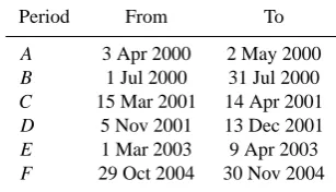
Figure 1 exhibits Sym-H index during the selected dif-ferent periods (named from A toF). The basic character-istic of the solar wind at 1 AU, as measured by L1 satellites (ACE/WIND), during each of the six selected time intervals are well described in Zhang et al. (2007). Each period can be divided into 3 subintervals, each characterized by either low, moderate or intense geomagnetic activity, respectively.
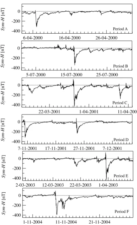
We apply the EMD, as described in Sect. 2, to the selected time series to separate them into their corresponding IMF. As example of our analysis, Fig. 2 reports the obtained IMFs relative to the Sym-H index from 1 July 2000 to 31 July 2000 (periodB).
As a result of the decomposition, one can see that the char-acteristic scale of each IMF increases with the mode indexk
and that there is a general separation of the data into locally non-overlapping time scale components. We recall that the number of IMFs can vary depending on the algorithm used to implement EMD. In particular, as already mentioned in Sect. 2, the critical point is represented by the stopping cri-terion. However, being the EMD decomposition is a sort of diadic filter bank (Flandrin et al., 2004), it is reasonable to expect a number of IMFs of the order of log2(N ), whereN
Period A
Period B
Period C
Period D
Period E
Period F -400
-200 0
Sym-H
[nT]
6-04-2000 16-04-2000 26-04-2000
-400 -200 0
Sym-H
[nT]
5-07-2000 15-07-2000 25-07-2000
-400 -200 0
Sym-H
[nT]
22-03-2001 1-04-2001 11-04-2001
-400 -200 0
Sym-H
[nT]
2-03-2003 12-03-2003 22-03-2003 1-04-2003 -400
-200 0
Sym-H
[nT]
7-11-2001 17-11-2001 27-11-2001 7-12-2001
-400 -200 0
Sym-H
[nT]
1-11-2004 11-11-2004 21-11-2004
Fig. 1. 1-min Sym-H(t) time series of the six selected time periods.
an energy-weighted measurement of the mean frequency in Fourier space.
However, to better analyze the dynamic response of the magnetosphere to the solar wind changes we separate the original signal and the obtained IMFs into three subinter-vals (I, II, III) of about 10 days (see vertical lines reported in Fig. 2), characterized by different geomagnetic activity lev-els. As a measure of the activity level characterizing each subinterval, we have considered the maximum jump in the Sym-H index according to the following expression:
δSym-H(t )=(Sym-H|max−Sym-H|min)T. (4) For each selected subintervalT (T = I, II, III), we estimate the mean frequencyhfkiof each modekas
hfki =
R+∞
−∞ f Sk(f )df R+∞
−∞ Sk(f )df
, (5)
whereSk(f )is the Fourier spectrum of IMFk (Huang et al.,
1998).
-150 15 IMF1 [nT]
-150 15 IMF2 [nT]
-150 15 IMF3 [nT]
-150 15 IMF4 [nT]
-150 15 IMF5 [nT]
-150 15 IMF6 [nT]
-150 15 IMF7 [nT]
-400 40 IMF8 [nT]
-150 15 IMF9 [nT]
-150 15 IMF10 [nT]
-400 40 IMF11 [nT]
-400 40 IMF15 [nT]
-400 40 IMF14 [nT]
-400 40 IMF12 [nT]
-400 40 IMF13 [nT]
-300 -1500 Sym-H [nT]
I II III
-400 40 IMF18 [nT]
-400 40 IMF19 [nT]
-400 40 Res [nT]
01/07/2000 08/07/2000 15/07/2000 22/07/2000 29/07/2000 Time
-400 40 IMF17 [nT]
-400 40 IMF16 [nT]
Fig. 2. From top to bottom: Sym-H time series for the time period B, from 1 July 2000 to 31 July 2000; 19 IMFs and residue resulting from EMD. Vertical lines denote the separation into three subin-tervals (I, II, III). The characteristic scale increases with the mode numberk.
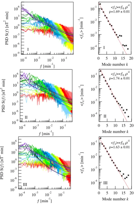
In Fig. 3, the Fourier spectra for all the IMFs are plotted on a double-logarithmic scale (left side) together with the estimated mean frequency of each IMF mode (right side) for the three different time intervals.
The relation between the indexkof the IMF and its mean frequencyhfkisuggests the following exponential law:
10-9 10-6 10-3 100 103 106
PSD S(ƒ) [nT
2 min]
10-4 10-3 10-2 10-1 ƒ [min-1] I
10-9 10-6 10-3 100 103 106
PSD S(ƒ) [nT
2 min]
10-4 10-3 10-2 10-1
ƒ [min-1] II
10-9
10-6
10-3
100
103
106
PSD S(ƒ) [nT
2 min]
10-4 10-3 10-2 10-1
ƒ [min-1]
III
20 15 10 5 0
Mode number k
10-4
10-3
10-2
10-1
<ƒ
k
> [min
-1 ]
I
<ƒk>=ƒ0
-k
=1.69 ± 0.01
20 15 10 5 0
Mode number k
10-4 10-3 10-2 10-1
<ƒ
k
> [min
-1 ]
II <ƒk>=ƒ0
-k
=1.74 ± 0.01
20 15 10 5 0
Mode number k
10-4
10-3
10-2
10-1
<ƒ
k
> [min
-1 ]
III
<ƒk>=ƒ0 -k =1.63 ± 0.01
Fig. 3. On the left: Fourier spectrum of all IMFs (from 1 to 19)
obtained by EMD for the three subintervals into which periodB
has been divided (I: 1–9 July 2000; II: 10–18 July 2000; III: 19– 31 July 2000, (from top to bottom). On the right: representation of the mean frequency vs. indexkin a log-linear view.
wheref0is a constant andρis given by the slope of the lin-ear fit performed in the semi-log representation of log(hfki)
vs.k. This result implies that the mean frequencyhfkiof a
given mode isρtimes larger than the mean frequency of the next one. In our case, taking into account the first ten mean frequency values, we obtainedρvalues that are significantly different from 2, which would correspond to a dyadic filter bank as obtained for white noise (Wu and Huang, 2004) and fractional Gaussian noise (Flandrin and Goncalv`es, 2004; Flandrin et al., 2004). Taking into account that the lowerρ
is, the larger the number of scales involved in the description of a phenomenon, we can considerρas a measure of the sig-nal multi-scale features and complexity. On the other hand, it has also been shown that departures ofρ from the value expected for stochastic noises (i.e.ρ=2) are observed in the case of intermittent turbulence, whereρis significantly lower than 2.
2.2 2.1 2.0 1.9 1.8 1.7 1.6 1.5
r
600 500 400 300 200 100 0
dSym-H [nT]
Increasing Complexity
Fig. 4. Dependence ofρ on δSym-H(t ). Colors refer to different time intervals: red to pre-storm time intervals, green to storm time intervals, and purple to after-storm time intervals.
For the above reason, it is interesting to analyze the de-pendence ofρ on the overall variation of Sym-H. Thus, we repeat the previous analysis for the other selected periods (see Table 1). First of all, we apply the EMD methodology to the original data of Sym-H in order to understand how the full spectrum process is split into its intrinsic mode func-tions. Secondly, we divide the original signal and its IMFs into three subintervals of the same length. For each interval, we estimate the mean frequency of each IMF and succes-sively we determine the value ofρ. The obtained results are reported in Fig. 4, where it is possible to evaluate the trend ofρas function of different levels of geomagnetic activity as described byδSym-H.
The diagram suggests that the complexity and the multi-scale nature of the magnetospheric response to the solar wind forcing is higher for intermediate values of δSym-H (from 150 nT to 300 nT) than for the other cases. In other words, the multi-scale features are a function of the geomagnetic ac-tivity level. Being the diagram of Fig. 4 represents the major result of our multi-scale analysis, the detailed discussion of this figure is postponed to the next section.
4 Discussion and conclusions
In the present study, we have analyzed the multi-scale fea-tures of a set of large geomagnetic storms by applying the EMD technique as introduced by Huang et al. (1998). The EMD analysis has emphasized the multi-scale and complex nature of the geomagnetic field fluctuations during large geo-magnetic storms. This point is corroborated by the high num-ber of intrinsic mode functions necessary to decompose the considered Sym-H time series.
suggests that the information content of the storm time sig-nal is higher than one of purely stochastic noise, and that the multi-scale features are more relevant. This is closely re-flected in the values ofρ, which are lower than 2. According to Huang et al. (2008), this higher number of IMFs could be due to the intermittent features of the investigated time se-ries. Indeed, intermittency is the counterpart of a more com-plex behavior, which involves non-trivial scaling features and perhaps a higher number of scales.
Our major result is reported in Fig. 4 where the depen-dence of ρ on δSym-H is shown. Considering the ρ pa-rameter as a sort of measure of the multi-scale character of the observed fluctuations, the plot seems to suggest that the multi-scale nature assumes a maximum value during time in-tervals characterized by intermediateδSym-H values. Tak-ing into account thatρ has been obtained from the depen-dence ofhfki onkat frequencies≤10−3min−1, the
multi-scale nature of fluctuations refers to typical time multi-scales below 1000 min (below 1 day). Thus, the increase of the multi-scale nature of Sym-H is maximum for medium to large geomag-netic activity, while it is reduced in the case of extreme geo-magnetic storm events.
In a recent study on storm–substorm relationship (De Michelis et al., 2011), it has been demonstrated that the influence (in terms of information flows) of substorms on storms is maximum in the case of moderate/intermediate ge-omagnetic activity level. In particular, during intense netic storms, which are mainly caused by an enhanced mag-netospheric convection following a long-lasting period of southward interplanetary magnetic field conditions (Kamide, 1992; McPherron, 1988), the driving of storms by substorms seems to be less effective. On the other hand, in several pa-pers it has been widely documented how the magnetospheric dynamics in the course of magnetic substorms shows dynam-ical complexity and an inherent multi-scale nature (e.g. Con-solini and Chang, 2001; Chang et al., 2003; Klimas et al., 2000; Lui et al., 2000; Chapman and Watkins, 2001).
The above considerations permit us a physical interpreta-tion of the results plotted in Fig. 4 in terms of the relevance of internal dynamics with respect to externally-driven enhanced convection. To fully understand and correctly interpret the re-sults reported in Fig. 4, we remind that Sym-H essentially de-scribes the ring current dynamics, and consequently we have to properly examine all those phenomena that are related to substorms and considerably influence this current system. In-deed, we can suppose that during a moderate activity level the internal magnetospheric dynamics are strongly affected by the impulsive and bursty character of plasma transport in the equatorial magnetotail regions (De Michelis et al., 1999). This plasma transport process, which is responsible for the substorm related phenomena, has been shown to be char-acterized by a strong intermittent coherent character (Con-solini and Chang, 2001; Chang et al., 2003; Klimas et al., 2000). This might be why the multiscale character becomes highly relevant during periods of moderate geomagnetic
ac-tivity. In contrast, during low and high geomagnetic activity levels, the geomagnetic field fluctuations seem to be a con-sequence of a very stochastic dynamics, similar to the global dynamics that characterize a Markovian nonequilibrium re-laxation process (e.g. de Groot and Mazur, 1984). This in-terpretation is also in agreement with the range of scales where the increment of the multi-scale nature is observed, being these scales are those typical of substorm events. In other words, the increase of the multi-scale nature during moderate activity levels reflects the influence of substorms to storms that is maximum during these periods. We can un-derstand this point by considering the different roles played by two main processes: the overall magnetospheric plasma convection and the impulsive relaxation events observed in the magnetotail regions, which are responsible for the geo-magnetic disturbances during different geogeo-magnetic activity levels. We can suppose that during low-to-moderate geomag-netic activity periods the observed geomaggeomag-netic fluctuations are dominated by the impulsive relaxation events that dom-inate the substorm dynamics, while during periods of high geomagnetic levels the fluctuations and the internal magneto-spheric dynamics are principally dominated by the enhance-ment of the overall plasma convection. This interpretation is also corroborated by the results on the nonequilibrium phase transition nature of the magnetospheric dynamics in response to solar wind changes, which displays both first and second order features (Sitnov et al., 2000, 2001).
In conclusion, this preliminary study indicates the inher-ent multi-scale nature of the magnetospheric dynamics dur-ing large storm events and its dependence on the overall geo-magnetic disturbance level. Clearly, more work is necessary to confirm these results on a larger survey of data.
Acknowledgements. We acknowledge the Kyoto World Data Center for providing Sym-H index time series used in the present study.
Edited by: B. Tsurutani
Reviewed by: A. C.-L. Chian and A. L. Clua de Gonzalez
References
Chang, T., Tam, S. W. Y., Wu, C. C., and Consolini, G.: Com-plexity, forced and/or self-organized criticality, and topological phase transitions in space plasmas, Space Sci. Rev., 107, 425– 445, 2003.
Chapman, S. C. and Watkins, N. W.: Avalanching and self organised criticality: a paradigm for magnetospheric dynamics?, Space Sci. Rev., 95, 293–307, 2001.
Consolini, G. and Chang, T.: Magnetic field topology and criticality in geotail dynamics: Relevance to substorm phenomena, Space Sci. Rev., 95, 309–321, 2001.
and the fluctuation theorem, J. Geophys. Res., 113, A08222, doi:10.1029/2008JA013074, 2008.
de Groot, S. R. and Mazur, P.: Non-equilibrium thermodynamics, Dover Publications Inc., New York, 1984.
De Michelis, P., Daglis, I. A., and Consolini, G.: An average image of proton plasma pressure and of current systems in the equato-rial plane derived from AMPTE/CCE-CHEM measurements, J. Geophys. Res., 104, 28615–28624, 1999.
De Michelis, P., Consolini, G., Materassi, M., and Tozzi, R.: An information theory approach to storm-substorm relationship, J. Geophys. Res., 116, A08225, doi:10.1029/2011JA016535, 2011. Dessler, A. and Parker, E. N.: Hydromagnetic theory of
geomag-netic storms, J. Geophys. Res., 64, 2239–2259, 1959.
Flandrin, P. and Goncalv`es, P.: Empirical mode decompositions as data driven wavelet-like expansions, Int. J. Wavelets, Multires. Info. Proc., 2, 477–496, 2004.
Flandrin, P., Rilling, G., and Goncalv`es, P.: Empirical mode de-composition as a filter bank, IEEE Sig. Proc. Lett., 11, 112–114, 2004.
Gonzalez, W., Joselyn, J., Kamide, Y., Kroehl, H., Rostoker, G., Tsurutani, B., and Vasyliunas, V.: What is a Geomag-netic Storm?, J. Geophys. Res., 99, A4, doi:10.1029/93JA02867, 1994.
Huang, N. E. and Wu, Z.: A review on Hilbert-Huang Transform: Methods and its applications to geophysical studies, Rev. Geo-phys., 46, RG2006, doi:10.1029/2007RG000228, 2008. Huang, N. E., Shen, Z., Long, S.,R., Wu, M. C., Shih, S. H., Zheng,
Q., Tung, C. C., and Liu, H. H.: The empirical mode decompo-sition and the Hilbert spectrum for nonlinear and non-stationary time series analysis, Proc. Royal Soc. A-Math. Phys., 454, 903– 993, doi:10.1098/rspa.1998.0193, 1998.
Huang, N. E., Wu, M. C., Long, S. R., Shen, Z., Qu, W., Gloersen, P., and Fan, K. L.: A confidence limit for the empirical mode decomposition and Hilbert spectral analysis, Proc. Royal Soc. A-Math. Phys., 459, 2317, doi:10.1098/rspa.2003.1123, 2003. Huang, Y. X., Schmitt, F. G., Lu, Z. M., and Liu, Y. L.: An amplitude
frequency study of turbulent scaling intermittency using Empiri-cal Mode Decomposition and Hilbert Analysis, Europhysics Let-ters, 84, 40010, doi:10.1209/0295-5075/84/40010, 2008. Iyemori T., Araki, T., Kamei, T., and Takeda, M.: Mid-latitude
geo-magnetic indices ASY and SYM (Provisional), Data Anal. Cent. for Geomagn. and Space Magn., Faculty of Sci., Kyoto Univ., Kyoto, Japan, 1992.
Kamide, Y.: Is substorm occurrence a necessary condition for a magnetic storm?, J. Geomagn. Geoelectr., 44, 109–117, 1992. Kamide, Y. and Maltsev, Y. P.: Geomagnetic Storms, in: Handbook
of the Solar-Terrestrial Evironment, edited by: Kamide, Y. and Chian, A., Springer-Verlag, Berlin Heidelberg, 2007.
Klimas, A. J., Valdivia, J. A., Vassiliadis, D., Baker, D. N., Hesse, M., and Takalo, J.: Self-organized criticality in the substorm phe-nomena and its relation to localized reconnection in the magneto-spheric plasma sheet, J. Geophys. Res., 105, 18765–18780, 2000. Lui, A. T. Y., Chapman, S. C., Liou, K., Newell, P. T., Meng, C. I., Brittnacher, M., and Parks, G. D.: Is the dynamic magnetosphere an avalanching system?, Geophys. Res. Lett., 27, 911–914, 2000. McPherron, R. L.: The role of substorms in the generation of mag-netic storms, in: Magmag-netic Storms, Geophys. Monogr. Ser., vol. 98, pp. 131–147, edited by: Tsurutani, B. T., Gonzalez, W. D., Kamide, Y., and Arballo, J. K., AGU, Washington D.C., 1988. Sckopke, N.: A general relation between the energy of trapped
par-ticles and the disturbance field near the Earth, J. Geophys. Res., 71, 3125–3130, doi:10.1029/JZ07i013p03125, 1966.
Sitnov, M. I., Sharma, A. S., Papadopoulos, K., Vassiliadis, D., Val-divia, J. A., Klimas A. J., and Baker, D. N.: Phase transition-like behavior of the magnetosphere during substorms, J. Geophys. Res., 105, 12955–12974, doi:10.1029/1999JA000279, 2000. Sitnov, M. I., Sharma, A. S., Papadopoulos, K., and
Vas-siliadis, D.: Modeling substorm dynamics of the magneto-sphere: From self-organization and self-organized criticality to nonequilibrium phase transitions, Phys. Rev. E, 65, 016116, doi:10.1103/PhysRevE.65.016116, 2001.
Vassiliadis, D.: Systems theory for geospace plasma dynamics, Rev. Geophys., 44, RG2002, doi:10.1029/2004RG000161, 2006. Wanliss, J. A. and Showalter, K. M.: High-resolution global storm
index: Dst versus Sym-H, J. Geophys. Res., 111, A02202, doi:10.1029/2005JA011034, 2006.
Wu, Z. and Huang, N. E.: A study of the characteristics of white noise using the empirical mode decomposition method, P. Roy. Soc. A-Math. Phy., 460, 1597–1611, 2004.
Zhang, J., Richardson, I. G., Webb, D. F., Gopalswamy, N., Hut-tunen, E., Kasper, J. C., Nitta, N. V., Poomvises, W., Thomp-son, B. J., Wu, C.-C., Yashiro, S., and Zhukov, A. N.: Solar and interplanetary sources of major geomagnetic storms (Dst ≤ −100 nT) during 1996–2005, J. Geophys. Res, 112, A10102, doi:10.1029/2007JA012321, 2007.