www.ocean-sci.net/6/211/2010/
© Author(s) 2010. This work is distributed under the Creative Commons Attribution 3.0 License.
Ocean Science
Variability of scaling time series in the Arctic sea-ice drift dynamics
A. Chmel1, V. N. Smirnov2, and I. B. Sheikin2
1Ioffe Physico-Technical Institute, Russian Academy of Sciences, 194021 St. Petersburg, Russia 2Arctic and Antarctic Research Institute, 38 Bering str., 199397 St. Petersburg, Russia
Received: 2 June 2009 – Published in Ocean Sci. Discuss.: 21 July 2009
Revised: 31 December 2009 – Accepted: 14 January 2010 – Published: 9 February 2010
Abstract. The motion of an individual ice floe in the Arctic Ocean was monitored at the Russian research station North Pole 35 established on the ice pack in 2008. The ice floe speed (V )was found to be correlated with wind speed (v)in main features, such as the positions of maxima and minima ofV andv. However, the fine structure of the V-variation cannot be explained by the wind forcing alone. There were periods of time when the floe drift was affected by the inter-actions of ice floes between each other or by the periodical forcing due to either the Coriolis inertia effect or the tidal ac-tivity. These data were compared with the “waiting times” statistics that are the distributions of time intervals between subsequent, sufficiently strong changes in the kinetic energy of drifting ice floe. These distributions were measured in several time windows differing in the average wind speed and wind direction, and/or in the mechanical state of the ice pack. The distribution functionsN (t > τ), whereN is the number of successive events of energy change separated by the time intervalt that exceeds τ, constructed in different time windows demonstrate fractal or a multifractal nature of the time series during motion in the consolidated ice pack but were truly random when the ice floe drifted in the highly fragmented sea ice. The latter result shows the existence of a relationship between the long-range mechanical interactions in the pack and long-term memory (time scaling behaviour) of the sea-ice motion.
1 Introduction
Recent studies of the sea-ice drift and mechanical behaviour of the ice pack, including its deformations and fragmenta-tions, revealed that the Arctic sea-ice cover (ASIC) exhibits well-pronounced scaling properties typical for the dynamics of non-equilibrium, permanently critical systems (Marsan et
Correspondence to: A. Chmel
al., 2004; Korsnes et al., 2004; Chmel et al., 2007; Ram-pal et al., 2008). The spatial, energy and temporal distribu-tions of mechanical events in the ASIC follow a power law with varying exponents, thus, indicating the existence of a la-tent relationship between the scaling features and underlying physical processes.
We can compare this behaviour of sea ice to the field of seismology where the temporal invariance of geophysi-cal processes is highly debated (Bak et al., 2002; Davidsen and Goltz, 2004; Varotsos et al., 2006; Telesca and Lovallo, 2008), because the recurrence time between earthquakes is the key parameter of the problem of catastrophe forecasting. Studying the time correlation of time events that take place within the ASIC, where the sea-ice floes have a high sim-ilarity to tectonic formations, allows one to establish some common trends in the behaviour of large-scale systems and to obtain new knowledge on the role of the time correlation in geophysics.
There were some previously reported (Chmel et al., 2005; Chmel et al., 2007) time characteristics of the sea-ice drift in the Arctic Ocean, as was revealed by the field observa-tions that were carried out at the research station “North Pole 32” (NP 32) established on the ice pack in 2003–2004. The sequence of events of accelerations of an individual ice floe was found to be self-similar (or, in terms of the critical dy-namics, fractal) during quasi-stationary periods of drift and fully disordered (truly random) when the great pack fragmen-tation occurred in the region of the NP 32 activity. The field investigation of the nonlinear sea-ice drift dynamics was con-tinued at stations NP 33 and NP 35 where the data of sea-ice motion were collected during 2005 and 2008, respectively. In this study, we present the original data recorded at these stations and the analysis of the ice floe motion during differ-ent periods of time. A particular attdiffer-ention was paid to the response of the drift dynamics to the varying external con-ditions, such as the wind forcing, inertia motion and sea-ice floes interactions. The cases of monofractal, multifractal and random time series are considered in the context of relative significance of physical processes that govern sea-ice drift.
2 Experimental technique and data processing
The permanent motion of the ice-pack consists of an infinite sequence of events of displacements mainly caused by wind forcing (Martin and Drucer, 1991) and, to a lesser extent, by ocean currents, which transform, at least partially, the direct force interactions between the sea-ice cover components. In-teractions of all kinds cause the local speed changes of indi-vidual ice floes, that is, the sea-ice floes limited by leads and cracks. In this work, the local speed changes were derived from the data on the ice floe displacements measured using GPS transmitters that were placed on the same ice floe at the same time at a distance of about 180 m. The data from two transmitters were collected using a field PC in sampling in-tervals of one minute. The observation accuracy when using GPS transmitters is given by the Twice the Distance Root Mean Square (2DRMS) error. The 2DRMS error refers to a horizontal distance that gives the radius of a circle/ellipse, which is centered on the true position and within 95% of all observed positions are located. The elongation of the ellipse is a measure for the quality of the position solutions derived by the GPS instrument. In the following, we shall denote the GPS transmitters as “master” and “slave” referring to their respective operational setting.
Figure 1 shows the positions measured with the slave transmitter in orthogonal coordinates centered at the posi-tion of the master transmitter and the respected 2DRMS. The shaded (grey) area shows a difference between two one-component statistics and a single two-component statis-tic in the local orthogonal coordinate system. The el-lipse is constructed using the compatible function of the two-dimensional probability distribution of pseudo distances with, taking into account, a correlation of the orthogonal measurements. Two semiaxes of 6.2 m and 4.0 m charac-terise the 2DRMS along the main directions.
In order to obtain estimates for the non-correlated mea-surement errors of the drift speed, as well as to assess their dependence of a sampling interval, the regression analysis of the data from two GPS transmitters situated at the distance of about 180 m was performed. The distances between se-quent measurement points in the sampling interval were used as the input data of the regression, and the standard error of the regression was taken as an estimate for the drift speed measurement error. Table 1 presents the obtained estimates for the standard error of regression, the non-correlated errors of the drift speed measurements and the errors of the calcu-lation rounding-off in different measurement intervals. The estimates show a significant decrease of the non-correlated noises with the decrease of the measurement interval and, in fact, this trend does not depend on the drift speed (Fig. 2). One can suppose that this behaviour is caused by the in-crease of the stability of the navigational satellites configu-ration with reducing the measurement interval. In addition, the data in Table 1 indicate that the rounding-off errors dom-inate in short measurement intervals.
10 Fig. 1
Fig. 1. 24-hour scattergram of the slave transmitter data presented in the local orthogonal coordinates. The ellipse (a) shows the 2DRMS (95% concentration) for the compatible function; (b, c): the fre-quency histograms of partial pseudo distance distributions with nor-mal approximations and partial standard deviations. (The pseudo distance, as distinct to the true distance, is a distance as measured
by a couple of GPS receivers with a relevant error.) 11
Fig. 2
Fig. 2. Standard error estimates of the drift speed. Sampling interval is 1 min.
Provided that the current geographical coordinates are known, the ice floe speed,V, can be calculated. Correspond-ingly, the speed changes, 1V, were determined in regular intervals1t=1 min.
Table 1. Sampling interval influence on the empirical error esti-mates*.
Sampling interval, min 1 2 5 10 Standard error of regression, m 0.8 1.14 1.62 1.91 Standard error of speed, m/sec 0.013 0.009 0.005 0.003 Rounding error m/sec 0.031 0.015 0.006 0.003
* For more detailed accuracy analysis of this experiment see (Sheikin and Smirnov, 2008).
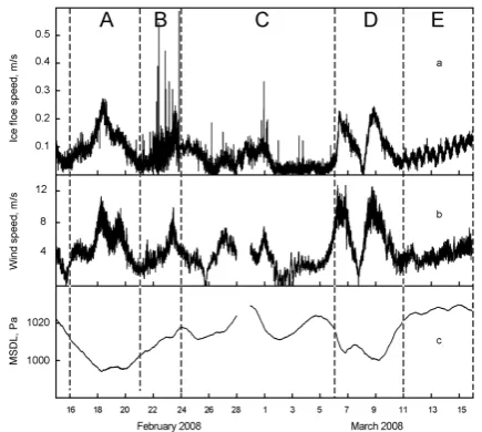
Figure 3a shows the ice floe drift speed measured from 16 February 2008 to 15 March 2008. This time interval was selected for analysis because it covers a few periods with quite a different character of the ice motion. Figure 3b and c characterise the main synoptic conditions, that is the wind speed and the MSLP, respectively.
The kinetic energy change,1E, is directly proportional to the speed change squared of the ice floe,1E∝1V2; here 1V2= |V02−V002|, whereV0andV00are the ice floe speeds measured in two subsequent time intervals (to simplify for-mulae, we shall denote1EasEhereinafter). Thus, a set of 1V2variations represents the time sweep of energy changes (Fig. 4). Only the values1V that exceeded the standard error of speed (Table 1) 5 times or more were taken into account in the subsequent data analysis. The percentage of such speed change values,1V > 1Vcut−off, was about 50% of all
mea-sured values. The time intervals between the events of speed change whose amplitude exceeded1Vcut−off were regarded as waiting times for the nearest sufficiently large event. A set of so derived waiting times was used to obtain the distribu-tion funcdistribu-tionN (t > τ )whereNis the number of successive “important” events separated by the time intervalt that ex-ceedsτ.
3 Results
3.1 R/Sanalysis
To assess the statistical correlation between events charac-terised by the energy change, that is to verify if there exists a dynamical connectedness of the drift as the physical pro-cess, a so-calledR/Sanalysis was applied to the sequence of events shown in Fig. 4. This statistical method is based on the determination of the ratio between the rangeR(N )and the dispersionS(N )defined as
R(N )= max 1≤j≤N
j X
i=1
(Ei−E)− min
1≤j≤N j X
i=1
(Ei−E) (1)
S(N )=
v u u t
N X
i=1
(Ei−E)2 (2)
12 Fig. 3
Fig. 3. Wind speed (a), ice floe speed (b), and Mean Sea Level Pressure data (c) during the time between 16 February to 15 March 2008. Gaps in (b) and (c) are due to instrumental failure. Top lettering between dashed lines denote five periods of observa-tion.
13 13
Fig. 4
Fig. 4. Amplitudes of kinetic energy changes found from the ice floe speed data obtained in the time interval 16 February to 15 March 2008.
whereN andEare the numerical length and the mean value of sequenceEi in a time windowτ, respectively. The
se-quence R/S behaves as a power law, R/S∝τH, where H is the Hurst exponent. H lies between the values 0 and 1; H >0.5 corresponds to positive correlation in the sequence of events: the largerτ, the more probable the further devel-opment of the process in the same direction;H <0.5 char-acterises an “anti-persistent” behaviour: a trend in dynamics that was established in the past will not continue in future; H=0.5 signifies the Gaussian random sequence.
14 Fig. 5
Fig. 5.R/Sanalysis dataset. The straight lines show the power law
R/S∝τH with different values ofH.
The valueH for the time series of energy changes shown in Fig. 3 was found from the slope of theR/Sversusτ depen-dence plotted in doubly logarithmic coordinates (Fig. 5). The valueH=0.96 in a time range of about 10 hours indicating a highly persistent trend (fractal ice floe motion); at largerτ the value ofHdecreases down to 0.62 (with significant vari-ations), and transverses the value 0.5 atτ≈102h. Thus, the time correlation radius of events was about four days.
3.2 Waiting time distribution
The “quiescent periods” between sufficiently large events (1V > 1Vcut−off)formed the times of waiting for any near-est event that exceeds the cut-off determined through the speed change. The waiting time distribution function con-tains information on the scaling features in the time series of ice drift. To construct the functionN (t > τ )graphically, the number of waiting timestexceeding an arbitrary givenτ was plotted againstτ in doubly logarithmic coordinates. The level of discrimination (cut-off) affects the waiting time dis-tribution because the cut-off defines, in fact, a ratio between “short” and “long” waiting times: the higher the cut-off, the smaller portion of low-amplitude accelerations characterised by “short” intervals between them is taken into account. This is seen in Fig. 6, where theN (t > τ )versusτ dependences calculated with different cut-off values are shown for the whole analyzed period (from 16 February to 15 March).
In a wide range of cut-off percentage, theN (t > τ ) func-tion follow the power law
N (t > τ )∝τδ (3)
which is a fingerprint of the fractal nature of the given time sequence of events. At the same time, Fig. 6 demonstrates that theN (t > τ )function obtained using a low cut-off (here 73% of events included) does not exhibit the power law be-haviour. This effect is commonly recognized in the seis-mology: due to the attenuation processes, “small” (at the
15 Fig. 6
Fig. 6. Waiting time distributionsN (t > τ )constructed with dif-ferent levels of discrimination of the ice floe speed change in 1 min intervals. Values near curves denote percentage of events taken into account at the given cut-off. The straight lines are power law fits.
given scale level) events cannot provide range, long-term interactions needed to form a fractal (Olami et al., 1992; S´anchez et al., 2002). On the other hand, an excessively high cut-off (here 4% of events included) reduces the number of used events down to the level inappropriate for statistical pro-cessing. The 50% discrimination used in this work seems to be optimal.
A comparison of theV-variation with the data of the wind speed (v)in the same period of observations demonstrate a relationship betweenV andv in main features, such as the positions of maxima and minima (Fig. 3). However, the fine structure of V-variation cannot be explained by the wind forcing only. One can distinguish, at least, two periods of time when the floe drift was affected by the action of another source of forcing.
First, on 21–23 February 2008, the ice floe exhibited quite excited motion, whose actual variability was much stronger than the variability of the wind speed in the same period of time. The wind-independent “jumps” seem to be due to the local interactions between ice floes, such as stick-slips and shearing.
Second, on 11–16 March 2008, a cyclicV-variation with a period equal to 12 h took place. This periodicity could be related with the appearance of the ice motion governed either by the Coriolis inertia or by the tidal activity superimposed on the wind forcing. Both these phenomena produce 12 h cycles in the sea-ice speed, and it is quite difficult to distin-guish between them without special measurements. In any case, a motion of this kind is driven by a periodical power source which suggests an insignificant action of random forc-ing that provides scalforc-ing effects; this mode of drift one could expect for sea-ice floes with suppressed or lacking interac-tion between each other. The disappearance of a 12 h pe-riodical component in the autocorrelation function of drift,
A. Chmel et al.: Variability of scaling time series 215
16
Fig. 7
Fig. 7. A fragment of ice floe trajectory during the time that covered a large scale pack fragmentation revealed in NOAA satellite images (see Fig. 8). Arrows indicate prevailing wind directions. Geographic location is indicated in Fig. 8.
17 17
Fig. 8
Fig. 8. Fragments of the AVHRR images of the region of NP 35 drift obtained on 29 February (a) and 10 March (b) 2008.
which correlated in time with a cycle of sea-ice fragmenta-tion, was previously derived from the NP 32 database analy-sis (Chmel and Smirnov, 2007). Therefore, we suggested that an event of substantial sea-ice fragmentation took place dur-ing the period of time preceded 11 March, 2008. The most probable candidate for this event is the day of 8 March when a sharp change in the ice floe/wind speed (Fig. 3) and the drift direction (Fig. 7) occurred. This is confirmed by study-ing the satellite images of the region of interest. The image of 10 March reveals a highly fragmented sea-ice pattern of disconnected floes instead of the relatively consolidated pack seen in the image of 29 February (Fig. 8).
Thus, one can divide the whole period of observations into a few conventionally separated time windows charac-terised by particular drift conditions, that is window (A) from 16 to 20 February: “stationary” wind-driven drift; (B) 21 to 23 February: highly excited motion; (C) 24 February to 6 March: wind-driven drift; (D) 7 to 10 March: a cycle of sea-ice fragmentation; (E) 11 to 15 March: drift driven by prevailing periodical forcing. In order to estimate the re-sponse of the ice floe motion on varying conditions of drift, the sequence of measured 1V was divided into five time windows.
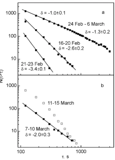
The obtained waiting time distributions for selected inter-vals are depicted in Fig. 9. The distributions are unambigu-ously different. In windows (A–D) theN versusτ depen-dence exhibits a power law with mono-exponent behaving in windows (A), (B) and (D); there is a dual exponent depen-dence in window (C).
The functionN (t > τ )does not follow the power law in window (E) (white squares in Fig. 9b).
4 Discussion
The power law decay of time correlations between physical events over wide time scales is typical for fractal behaviour inherent in permanently critical systems, that is in systems where correlations are much larger than the length scale of direct interaction.
The absolute value of the power exponent characterises the relative contribution of “short” and “long” waiting times to the wholeN (> τ )distribution. The largest absolute value of δ= −3.4 was obtained for window (B) (Fig. 9a) during the highly excited motion characterised by predominantly short recurrence times. Two different exponents equal to−1.0 and −1.3 characterise the ice floe motion in window (B). This means that the waiting time distribution is multifractal, that is the ice floe is involved into two critical processes of different
18 Fig. 9
Fig. 9. Waiting time distributionsN (t > τ )in different time win-dows in February (a) and in March (b) 2008.
time scale levels. Since the temporal characteristics of the permanently critical systems are interrelated with their spa-tial properties (Maslov et al., 1994; Rampal et al., 2008), one can suggest that the time multifractality is caused by the fact that the detected speed changes were corresponded with the simultaneous motion of sea-ice floes belonging ei-ther to different hierarchy levels, say, local and regional ones in terms of the classification by Overland et al. (1995), or to different mechanical processes, such as prevalent shearing and prevalent impact interactions, or to different components of anisotropic fracturing, etc.
The waiting time distribution measured in window E does not exhibit a log-linear dependence. In the light of the data presented in this work, we conclude that the loss of the tem-poral correlation occurred after the beginning of the fragmen-tation as a result of the multiple breakage of structural links in the fracturing sea-ice cover. In the current study, the pre-vailing regular motion in the period between 11 to 15 March (window E) signalizes the low interactions of the ice floe with neighbouring ice structures. The lack of long-range interac-tions excludes the possibility of long-term time correlainterac-tions since the structural memory of preceding events in a multi-component system is, in fact, a cooperative response of the system as a whole on the behaviour of its individual compo-nents. In our case, an ice floe itself does not store the infor-mation about its prehistory, while its environment, the floe field, does. The highly variable contact interactions (stick-slips, impact, etc.) play the role of dynamical structural links in the mobile ensemble of sea-ice floes.
The effect of the mechanical connectedness of the non-equilibrium statistical system on its scaling properties was considered in a number of model simulations (Christensen and Olami, 1992; Olami et al., 1992; Abaimov et al., 2007). A scenario close to our situation was analyzed by Abaimov et al. (2007) using a slider-block model for slip events. The au-thors concluded that the scale-invariant statistics of the recur-rence times depend on the system’s stiffness: the lower the stiffness (and, hence, the energy conservation), the smaller the size of elements that interact following the power law waiting time statistics. In a highly stiff system, the power law waiting time statistics cover the events of all spatial scale levels. The qualitative conclusion of this simulation – the lower the conservative properties of the system, the lesser pronounced its time scale invariant behaviour – is consistent with the loss of the time scaling during the relatively free drift of the ice floe observed in our study.
5 Conclusions
The length distributions of time intervals between subse-quent sufficiently strong changes in the speed of ice floe drifting in the consolidated pack demonstrate the power law behaviour. The values of the power law exponent are sensitive to the intensity of the wind forcing because the contribution of “short” and “long” time intervals to the waiting time distribution depends on the variability of the ice floe speed. However, in the highly fragmented sea-ice, the waiting-time statistics are no longer following a scale behaviour because the memory on the space-time trajectory of the low-connected, low-interacting system cannot be ef-ficiently maintained. The R/S (Hurst) analysis confirms the fractal nature of time sequences of kinetic energy changes occurring during the drift.
Edited by: D. Stevens
References
Abaimov, S. G., Turcotte, D. L., Sherbakov, R., and Rundle, J. B.: Recurrence and interoccurence behaviour of self-organized complex phenomena, Nonlin. Processes Geophys., 14, 455–464, 2007,
http://www.nonlin-processes-geophys.net/14/455/2007/. Bak, P., Christensen, K., Danon, L., and Scalon, T.: Unified
scaling law for earthquakes, Phys. Rev. Lett., 88(1-4), 178501, doi:10.1103/PhysRevLett.88.178501, 2002.
Chmel, A. and Smirnov, V. N.: The Arctic sea-ice cover: Problem of forecasting, Physica A, 375, 288–296, 2007.
Chmel, A., Smirnov, V. N., and Astakhov, A. P.: The Arctic sea-ice cover: fractal space-time domain, Physica A, 357, 556–564, 2005.
Chmel, A., Smirnov, V. N., and Panov, L. V.: Scaling aspects of the sea-ice-drift dynamics and pack fracture, Ocean Sci., 3, 291– 298, 2007,
http://www.ocean-sci.net/3/291/2007/.
Christensen, K. and Olami, Z.: Scaling, phase transitions, and nonuniversality in a self-organized critical cellular-automation model, Phys. Rev. A, 46, 1829–1838, 1992.
Davidsen, J. and Goltz, C.: Are seismic waiting time distributions universal? Geophys. Res. Lett., 31, L21612–L21616, 2004. Korsnes, R., Souza, S. R., Donangelo, R., Hansen, A., Paczuski,
M., and Sneppen, K.: Scaling in fracture and refreezing of sea-ice, Physica A, 331, 291–296, 2004.
Marsan, D., Stern, H., Lindsay, R., and Weiss, J.: Scale dependence and localization of the deformation of Arctic Sea-ice, Phys. Rev. Lett., 93(1–4), 178501, 2004.
Martin, S. and Drucer, R.: Observation of short-period ice floe ac-celerations during leg II of the Polarbjorn drift, J. Geophys. Res., 96, 10567–10580, 1991.
Maslov, S., Paczuski, M., and Bak, P.: Phys. Rev. Lett., 73, 2162– 2165, 1994.
Olami, Z., Feder, H. J. S., and Christensen, K.: Self-organized criti-cality in a continuous, nonconservative cellular automaton mod-eling earthquakes, Phys. Rev. Lett., 68, 1244–1247, 1992.
Overland, J. E., Walter, B. A. Curtin, T. B., and Turet, P.: Hierarchy and sea-ice mechanics: a case study from the Beaufort Sea, J. Geophys. Res., 100, 4559–4571, 1995.
Rampal, P., Weiss, J., Marsan, D., Lindsay, R., and Stern, H.: Scaling properties of sea-ice deformation from buoy dispersion analysis, J. Geophys. Res., 113(1-12), C03002, doi:10.1029/2007JC004143, 2008.
S´anchez, R., Newman, D. E., Carreras, B. A.: Waiting time statis-tics of self-organized-criticality systems, Phys. Rev. Lett., 88(1-4), 68302, doi:10.1103/PhysRevLett.88.068302, 2002.
Sheikin I. B. and Smirnov, V. N.: Accuracy estimation of the GPS measurements at the Russian drifting stations North Pole-33 and North Pole-35, Proc. 19t h IAHR International Symposium on Ice, Vancouver, Canada, July, 2008.
Telesca, L. and Lovallo, M.: Investigating non-uniform scaling behaviour in temporal fluctuations of seismicity, Nat. Hazards Earth Syst. Sci., 8, 973–976, 2008,
http://www.nat-hazards-earth-syst-sci.net/8/973/2008/.
Varotsos, P. A., Sarlis, N. V., Skordas, E. S., Tanaka, H. K., and Lazaridou, M. S.: Attevmpt to distinguish long-range temporal correlations from the statistics of the incre-ments by natural time analysis, Phys. Rev., 74(1-12), 021123, doi:10.1103/PhysRevE.74.021123, 2006.