Quantify the quantitative easing: impact on bonds and corporate debt issuance
LSE Research Online URL for this paper: http://eprints.lse.ac.uk/101665/ Version: Accepted Version
Article:
Todorov, Karamfil (2019) Quantify the quantitative easing: impact on bonds and corporate debt issuance. Journal of Financial Economics. ISSN 0304-405X
https://doi.org/10.1016/j.jfineco.2019.08.003
Reuse
This article is distributed under the terms of the Creative Commons Attribution-NonCommercial-NoDerivs (CC BY-NC-ND) licence. This licence only allows you to download this work and share it with others as long as you credit the authors, but you can’t change the article in any way or use it commercially. More information and the full terms of the licence here: https://creativecommons.org/licenses/
Quantify the Quantitative Easing: Impact on Bonds
and Corporate Debt Issuance
✩Karamfil Todorova,∗
a
OLD 3.02, Finance Department, the London School of Economics and Political Science, Houghton Street, London, United Kingdom, WC2A 2AE
August 2018
Abstract
This paper studies the impact of the ECB’s Corporate Sector Purchase Programme (CSPP) announcement on prices, liquidity and debt issuance in the European corporate bond market using a dataset on bond transactions from Euroclear. I find that the QE programme increased prices and liquidity of bonds eligible to be purchased substantially. Bond yields dropped on average by 30 bps (8%) after the CSPP announcement. Tri-party repo turnover rose by 8.15 million USD (29%), and bilateral turnover went up by 7.05 million USD (72%). Bid-ask spreads also showed significant liquidity improvement in eligible bonds. QE was successful in boosting corporate debt issuance. Firms issued 2.19 billion EUR (25%) more in QE-eligible debt after the CSPP announcement, compared to other types of debt. Surprisingly, corporates used the attracted funds mostly to increase dividends. These effects were more pronounced for longer-maturity, lower-rated bonds, and for more credit-constrained, lower-rated firms.
Keywords: Quantitative easing (QE), Corporate Sector Purchase Programme, European
Central Bank, bond market, corporate debt issuance
JEL Classification: E52, E58, G12, G18
1. Introduction
Recent years have seen a surge in the use of unconventional monetary policy tools across the developed world. Following the 2008 financial crisis, major central banks have exhausted the traditional monetary toolkit and have started using new instruments to spur economic activity and tackle low inflation. Being constrained by the (near zero) lower bound of interest rates, national regulators have expanded their traditional measures for stimulating the economy by conducting large-scale asset purchases known as quantitative easing (QE). Billions of dollars, euros, pounds and yen have been injected into the economy by the Federal Reserve (Fed), the European Central Bank (ECB), the Bank of Japan (BoJ), and the Bank of England (BoE) in order to buy bonds and other asset classes as part of QE. These massive purchases represent a
✩I would like to thank Ron Anderson, Simeon Djankov, Daniel Ferreira, Christian Julliard, Dong Lou, Igor
Makarov, Ian Martin, Martin Oehmke, Daniel Paravisini, Andrea Tamoni, Dimitri Vayanos, Kathy Yuan and Jean-Pierre Zigrand for their useful advice and comments. I am also grateful to seminar participants at the London School of Economics and Political Science, Goethe University Frankfurt, Paris Dauphine University, London Business School and EEA, Manchester for their helpful feedback.
∗Corresponding author
substantial fraction of the GDPs of these countries1, but despite its large scale, little research has been devoted to the consequences of QE for bond prices, liquidity and for corporates in general. In this paper, I exploit a unique dataset on bond transactions and firms’ financial indicators, which allows me to study questions as yet unanswered in the QE literature. I quantify the very heterogeneous effects of the European QE programme on bonds and on corporate debt issuance. Surprisingly, I find that the main effects of QE for corporates were transmitted through increase in dividend payments rather than through changes in investment. 1.1. Empirical evidence
The analysis developed in this research is based on the Corporate Sector Purchase Pro-gramme (CSPP) launched by the ECB in 2016 as part of QE. The focus of the study is on the ECB because of all the central banks implementing QE, the European institution is the largest holder of corporate bond debt2. This paper exploits the exogenous nature of the CSPP announcement to construct a before-after comparison between bonds that are eligible for pur-chase and bonds that are not. I make use of a proprietary data set on bond transactions between February 2015 and June 2016 from Euroclear, combined with pricing information from Bloomberg and with firms’ financial data from the Bureau van Dijk, and employ a difference-in-differences (DD) research design to estimate the causal impact of QE.
The first broad topic of this paper is the impact of QE on bond prices and liquidity. The results show that QE significantly increased prices: yields of eligible bonds declined by 30 bps (8%) after the CSPP announcement. The policy also had a large positive impact on liquidity, which I quantify using two main metrics: trading activity (turnover) and cost of trading (bid-ask spreads). After the CSPP announcement, tri-party (repo) turnover increased on average by 8.15 million USD (29%) and bilateral (buyer-seller) turnover3 went up by 7.05 million USD (72%). The bid-ask spread of yields went down by 46%, indicating massively reduced costs of a round-trip transaction. However, the positive impact on liquidity was mostly concentrated in the segment of QE-eligible bonds. The effects on ineligible bonds were less pronounced, and in the tri-party repo market, liquidity of these bonds even decreased after QE. Moreover, the initial spike in trading activity gradually dissipated. In contrast, the impact on yields and the reduction in trading costs were more persistent. There was also some evidence of spillover effects to yields of ineligible bonds.
As a next step, the paper studies which bonds benefited the most from the QE intervention. The drop in yields is decomposed into different risk premia by applying the methodology of Krishnamurthy and Vissing-Jorgensen (2011) (KVJ) [15]. I run DD regressions, splitting the sample of bonds into several maturity-rating-liquidity risk buckets to isolate the duration risk channel, the default risk channel and the liquidity channel of QE. The results show that the greatest effects of the CSPP were observed for bonds with higher duration and default risks. The estimates reveal an inverse relationship between the rating of a bond and the decline in
1
Around 20% for the Fed and the BoE, 40% for the ECB and more than 90% for the BoJ as of May 2017. Sources – the Fed, the ECB, the BoE, the BoJ.
2
170.38 billion euros as of September 2018. Source – the ECB. 3
A bilateral trade takes place when two member firms provide matching instructions to Euroclear to transfer ownership from one counterparty to the other in return for an agreed amount of money. The tri-party repo transactions are repurchase transactions arranged by a tri-party repo agent whereby one party may obtain short-term funds by providing a security it owns for a sale to a counterparty with a matching repurchase agreement set for a later date.
yields. A positive relationship is observed between the maturity of the bond and the reduction in yields: longer-duration bonds experienced the largest drop in yields. On the other hand, the liquidity impact of QE was only marginally different for bonds with different duration and default risks.
The fact that eligible lower-rated, longer-maturity bonds close to the threshold were the main drivers of the decrease in yields shows that the ECB’s intervention had a higher positive impact on riskier debt instruments within the treated set of bonds. These findings suggest that the European QE was successful in reducing the duration, the default and the liquidity premiums of eligible bonds and in re-allocating risks. The logic is as follows. In times of financial turmoil investors typically require a larger premium for holding riskier bonds, causing a decrease in bond prices. As a consequence, banks holding these risky illiquid bonds may become constrained by their risk bearing capacity as in Vayanos and Vila (2009) [20], or face VaR constraints. By implementing QE, the central bank steps in, inflates bond prices and improves liquidity by making it easier for investors to sell these risky illiquid assets as part of the bond buying programme, thereby reducing the risk premium and lowering bond yields. The drop in yields and the increase in liquidity could potentially reduce risks in the system by removing problematic assets from banks’ balance sheets and by contributing to deleveraging (see, e.g., Woodford, 2012 [21]). The effects of the European QE documented in this research are consistent with such a story.
The second broad part of this paper studies the reaction of corporates to QE. The analysis shows an overall increase in the issuance of QE-eligible bonds compared to ineligible ones both in the absolute number of bonds and in the par amount outstanding. However, firms issuing eligible bonds might be systematically different from those issuing ineligible bonds. To address this concern, I saturate the firm dimension by restricting the sample to firms that can issue bonds in both segments. If there was a switch to issuing more QE-eligible debt, these firms would be more likely to issue a larger amount of their debt liabilities in euro-denominated bonds that satisfy the CSPP criteria, and less in other types of bonds. This is indeed what I find. Corporates issued 1.39 QE-eligible bonds more per week, after the CSPP announcement, compared to ineligible bonds. This corresponds to 1.94 billion EUR, or a 49% rise in newly issued QE-eligible debt each week. Firms also increased the fraction of bond debt in their total liabilities.
Next, the study focuses on the heterogeneous effects of QE for firms with different risks. A number of papers (see, e.g., Kashyap et al., 1993 [13]; Rauh and Sufi, 2010 [16]) document the fact that corporates become more credit-constrained and reduce bank borrowing during financial crises. However, it is unclear, whether QE would alleviate the problem by boosting new debt issuance and easing borrowing for more financially constrained firms. It is also de-batable, whether these firms would use the funds attracted through bond issuance, to increase investment. To answer these questions, I conduct the following analysis. Given that longer-duration, lower-rated bonds experienced the largest drop in yields, one could hypothesize that firms would be more likely to issue bonds with longer maturities and that riskier firms would make wider use of the programme. To test these hypotheses, I split the eligible segment in different rating and maturity groups and run several DD regressions. The results show that corporates were indeed more likely to issue bonds with longer maturities. Moreover, the esti-mates illustrate a monotonic inverse relationship between the rating of a firm and the amount of issued QE-eligible debt. This fact shows that lower-rated corporates made wider use of the programme.
Surprisingly, however, the funds attracted through QE, were not used to increase invest-ment, but were mostly utilized through dividend payments. The results of a DD regression on a subset of firms with financial data before and after the CSPP announcement show that firms issuing QE-eligible bonds did not change cash holdings, investments in working capital, PPE or R&D. To the contrary, these firms increased dividends four times compared to the before-QE mean of firms not issuing QE-eligible bonds. These new empirical findings suggest that QE was successful in providing cheap liquidity to more credit-constrained corporates by lowering the cost of market debt issuance. However, the programme had greater impact on firms’ dividend payments and little impact on investment.
The main conclusions of this paper are verified in a series of robustness checks. To address the issue of heterogeneity in bond characteristics, I construct a matched sample, restricting the treatment group to bonds for which there is a suitable control bond with similar pre-treatment characteristics (par amount outstanding, rating, time to maturity). I also try different vari-ations of the control group and extensions of the post-announcement period. Furthermore, I collapse the data by time and run pure time-series tests to verify the panel regression es-timates. The main findings of the study are robust to these modifications. To check that the sample selection of bonds in treatment and control groups does not mechanically produce the main results, the study performs two placebo tests. In the first, the sample period is shifted backwards by 1 year to remove any effects of seasonality. In the second, USD denomi-nated bonds that satisfy all the CSPP eligibility criteria are used as a treatment group. Both placebo tests show no statistically significant effects and rule out the possibility that the main conclusions of the research are due to seasonality, or due to mechanical sample selection. 1.2. Related literature
The analysis developed in this paper is related to the growing literature on quantitative easing. Most articles in the QE literature have focused on the effects of the Fed’s QE pro-gramme. Krishnamurthy and Vissing-Jorgensen (2011) (KVJ) [15] study the impact of the Federal Reserve’s QE programmes on interest rates and outline several important channels through which QE affects bond yields. In a recent paper Song and Zhu (2018) [17] analyze the implementation of QE in the U.S. and study which bonds are more likely to be purchased by the Fed. Christensen and Gillan (2018) [7] find that the Federal Reserve’s second QE programme improved market liquidity. However, there is little research on the impact of the ECB’s QE on bond yields, liquidity, and on corporate debt issuance, partly because there is no analogue of the TRACE database for European bonds. Given the significance of the cor-porate bond market in Europe, however, the impact of the ECB’s QE is an important concern for European investors and market participants. To the best of my knowledge, the research presented here is the first one to analyze the impact of the European QE on bond yields and bond liquidity, and the first one to study firms’ reaction to QE in general.
This paper is also related to the literature on liquidity measures in financial markets. Asquith et al. (2013) [3] assess the impact of a mandatory transparency regulation on bond liquidity using volume of trading and turnover ratio. Amihud (2002) [2] develops a new price-volume indicator to measure liquidity in the stock market. Huang and Wang (2009) [11] show that illiquidity can lead to crashes in asset prices and increases in volatility. Bao et al. (2008) [4] confirm the latter conclusion and show that liquidity of corporate bonds decreased signif-icantly during the financial crisis of 2008. In recent research, Markit and the TABB Group (2016) [19] summarize the most commonly used measures of liquidity and show that liquidity
increased in the US corporate bond market after the financial crisis. In the research presented here, I contribute to the literature by quantifying the impact of QE on liquidity of European corporate bonds using turnover, bid-ask spreads and the Amihud illiquidity measure.
The paper presented here also builds on the extensive literature on corporate debt issuance. Bolton and Freixas (2000) [6] present a model in which, because of the greater flexibility of bank credit, corporates with higher default probability would prefer bank financing to bond financing during financial distress. Becker and Ivashina (2014) [5] find evidence that firms substitute bank credit with bonds as credit conditions tighten. Rauh and Sufi (2010) [16] find similar effects for US rated firms: corporates substitute bank credit with bond financing as their credit quality increases. The conclusions of De Fiore and Uhlig (2012) [8] are in line with these findings. Their paper shows how banking distress can lead to a surge in corporate bond issuance. The results of the research presented here complement the literature on cor-porate debt issuance. Consistent with the conclusions of Adrian and Shin (2012) [1], Becker and Ivashina (2014) [5] and De Fiore and Uhlig (2012) [8], I find that there is a switch to issuing more corporate debt in the aftermath of the financial crisis. The new result is that these conclusions continue to hold even during a QE intervention and in a low-interest rate environment. Moreover, I document that riskier firms issued more debt in response to QE implementation. I also find that corporates were more likely to issue longer-maturity bonds since QE reduced yields of these bonds the most.
Financial regulators and international finance associations have expressed differing views on the potential impact of the European corporate bonds purchase programme on debt is-suance. For example, in a note, the International Capital Market Association ICMA (April, 2016) [12] argues that cheaper funding opportunities due to the CSPP would not have a signif-icant influence on firms’ debt issuance, since “many corporates are already awash with cash”. The note also argues that the ECB’s intervention might in fact push investors towards more risky QE-ineligible bonds in the search for yield, and reduce liquidity in eligible bonds. On the other hand, Demertzis and Wolff (2016) [9], and Sparks (2017) [18] claim that there is evidence that corporates took advantage of the CSPP to issue a greater number of securities. There is no clear consensus on the effects of the CSPP for corporate debt issuance, bond prices, bond liquidity, and the use of QE funds. The research presented here aims to fill in these gaps.
The rest of this paper is organized as follows. In Section 2, I describe the data set, the research framework, and give details of the CSPP. Section 3 presents the results for the impact of the ECB’s intervention on bond prices and liquidity. Section 4 describes the corresponding results for corporate debt issuance and the use of QE funds. Section 5 presents two placebo tests and Section 6 concludes.
2. Data and Research Framework 2.1. Data
The data set used in this research consists of information on the total volume of trading (turnover) and the holdings of individual bonds reported by Markit based on reports supplied by Euroclear Plc. (the largest securities depository in the Eurobond market and a major clearing house). I combine this data with information on the issue, the issuing entity, and the price of each bond from Bloomberg, and with data on firms’ financial indicators from the Bureau van Dijk.
The Euroclear data set reports total daily transactions on individual securities from Febru-ary, 2015 to June, 2016. For each security (identified by ISIN) I observe the total value of transactions (expressed in USD equivalents) in the bilateral and tri-party repo market. The entire data set consists of 109 421 different ISINs and 330 trading days. As many bonds do not trade on a day-to-day basis, I construct total weekly turnover of a given bond, which is consistent with the literature on bond liquidity (see, e.g., Asquith et al., 2013 [3]). Since the focus of this paper is the impact of the CSPP on European corporate bonds, I filter out all non-corporate bonds, and all bonds outside the EU. This leaves a total of 6 590 bonds traded during the sample period. The next section provides details of the corporate bonds purchase programme.
2.2. The CSPP
The ECB started a series of QE-programmes following Mario Draghi’s famous “whatever it takes” speech in 2012. The first programmes, the ABSPP (Asset-Backed Securities Purchase Programme) and CBPP (Covered Bond Purchase Programme) were aimed at buying long-term EU sovereign bonds. These programmes improved economic conditions in the euro area and contributed to growth (see, e.g., Demertzis and Wolff, 2016 [9]), but were not enough to achieve the inflationary target set by the ECB. It became evident that the European regulator should go beyond government bonds and target riskier assets as part of its QE programme.
On 10 March 2016, the ECB announced a further expansion of its asset purchase pro-gramme including the new CSPP. This measure was introduced with its main purpose being to “further strengthen the pass-through of the Eurosystem’s asset purchases to the financing conditions of the real economy” and was expected to last until at least March 20174. The decision to include investment grade non-bank corporate bonds in the QE programme caught the market by complete surprise. The CSPP was a very novel measure since the ECB entered the private sector financing market, whereas previously it had bought almost exclusively gov-ernment bonds as part of QE. However, the full details of the CSPP, including the eligibility criteria, were not specified, with the promise of making them public “in due course”. In fact, this promise left more questions than answers, since it did not explicitly define the range of ratings, set of maturities, or firm eligibility criteria.
On 21 April 2016, the ECB published a full set of criteria for a bond to be purchased under the new programme. To be eligible, a bond had to satisfy the following conditions:
• be denominated in euros
• have a minimum rating of BBB-or equivalent
• have a remaining maturity of 6 months - 30 years at the time of purchase
• be issued by a corporation established in theeuro area; credit institutions not eligible.
The programme was scheduled to start at the beginning of June 2016. 2.3. Summary statistics
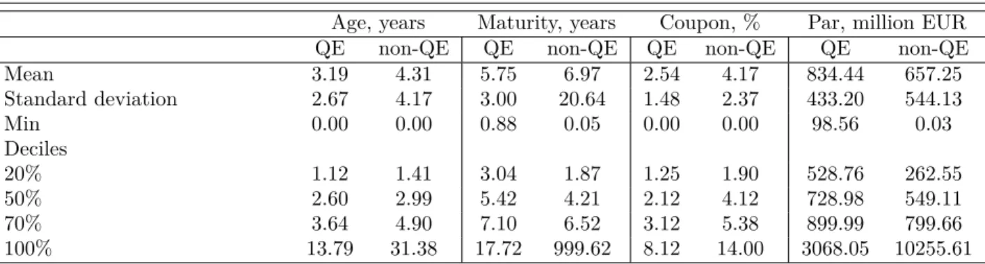
Table 1 and Figure 1 present summary statistics of the QE-eligible (546) and ineligible (6044) bonds.
4
[Table 1 and Figure 1 about here]
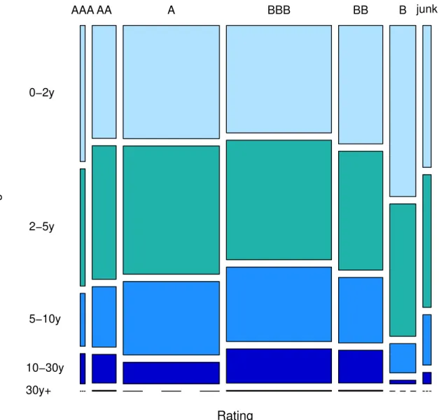
Figure 2 shows the age-rating distribution of the whole dataset for comparison. As we can see from Table 1, QE-eligible bonds (column QE) are on average younger and have larger amounts outstanding, compared to the ineligible ones (column non-QE). This is true for the mean and the median, and largely for the whole distribution (as seen from the deciles). In addition, QE-eligible bonds are always rated above BBB. This heterogeneity might be driving the differences in bond prices and liquidity. I address this issue in Section 3 of the paper.
[Figure 2 about here]
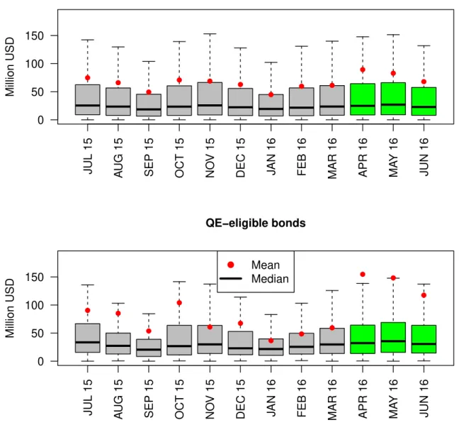
Figure 3 presents monthly summary statistics of the bilateral trading volume for all Eu-ropean corporate bonds and for the QE-eligible segment separately. As we can see, the dis-tribution of turnover is highly positively skewed, the mean being higher than the median. This is more pronounced for the QE-eligible segment where the difference is of the magnitude 2-4 times. Inspecting the quartiles also confirms the positive skewness, since even the third quartile is often lower than the mean. Table A.1 in the Appendix illustrates that a similar picture is observed for the tri-party repo market where the positive skewness is even stronger.
[Figure 3 about here]
Figure 3 illustrates also that the difference between the mean and the median trading volume starts to diverge for the last three green bars, particularly for the segment of QE-eligible bonds. This is the first evidence of increased trading in large quantities around March 2016. Presumably, it was the newly launched ECB’s QE programme that drove these results.
[Figure 4 about here]
The plots of bond yields and trading volume before and after the CSPP in Figure 4 support this hypothesis. Before the QE announcement, both bilateral and tri-party repo trading volumes move in parallel trends. However, after the CSPP, we see a large spike in turnover of QE-eligible bonds for both markets. At the same time, we see a drop in yields at time of the CSPP announcement and in the post-announcement period which suggests QE increased bond prices. To prove that the ECB’s intervention caused these changes, however, I test the causality in a more rigorous way using a regression approach.
2.4. Research framework
The empirical strategy in this research exploits the CSPP announcement to construct a before-after comparison between bonds that are eligible for purchase and bonds that are not. To study the impact of QE, I take a window around the announcement and employ a difference-in-differences research design. This methodology allows me to avoid confounding the effects of QE with unobserved shocks to the European corporate bond market. Figure 4 confirms that the parallel trends assumption for the DD specification is largely satisfied.
The sample period analyzed in this study is January 2016 to June 2016 (23 weeks). To the best of my knowledge, no other significant events influenced exclusively the European corporate bonds market in the sample period, so the main driver of changes in liquidity and debt issuance in this market was presumably the ECB’s intervention. The period between the announcement of the CSPP on 10 March 2016, and 21 April 2016 (the day when the criteria were revealed) is defined as the interim period, and the period after 21 April 2016 as
the post-announcement period. The corresponding regression dummies are Inter and Post. A bond is defined as being part of the treatment group if it satisfies all the CSPP eligibility criteria. The corresponding dummy variable is Treat. The basic regression specification is:
yit =αi+λt+γT reat×Inter ×T reati×Intert+γT reat×P ost×T reati×P ostt+ǫit, (1) where yit is the variable measuring yields (Yit), liquidity (e.g., T urnoverit, T urnover ratioit,
Bid-ask spreadit), firms’ debt issuance (e.g.,N umber of bondsit) or firms’ financial indicators
(e.g., Dit). αi is an individual (bond/firm) fixed effect and λt is a time fixed effect. In later
specifications, the basic regression is modified by adding controls and rating dummies. The next section studies the impact of the QE programme on bond prices and liquidity.
3. Impact of QE on Bond Prices and Liquidity
This part analyzes the first broad topic of the paper, namely, the effects of the ECB’s QE on bond prices and liquidity. To estimate the impact on prices, I look at changes in bond yields of eligible versus ineligible bonds after QE. To quantify the effect on liquidity, I measure it within two main dimensions: trading activity and cost of trading. The first one is estimated using weekly turnover (volume of trading) and turnover ratio (volume of trading scaled by the par amount of the bond) as they are commonly used indicators of trading activity in the bond literature (see, e.g., Asquith et al., 2013 [3]). The cost of trading aspect of liquidity is quantified using bid-ask spreads as they represent the cost of a round-trip transaction in raw terms.
Table A.2 in the Appendix also provides regression results using scaled bid-ask spreads: divided by either the bid price (sometimes referred to as the liquidity cost score LCS =
Ask−Bid
Bid ) or by the mid-price (the effective spread ES =
Ask−Bid
M id ). It also presents the results
for price impact indicators (the Amihud illiquidity measure) to quantify liquidity within a third dimension: the ease with which large quantities can be traded on the market. The main conclusions of this research also hold with these measures of liquidity.
First, I analyze the impact of QE on bond yields. Columns 1-3 of Table 2 estimate the basic regression (1) and a modification without time and bond fixed effects:
yit=α+γT reat×T reati+γInter×Intert+γP ost ×P ostt+
γT reat×Inter ×T reati×Intert+γT reat×P ost×T reati×P ostt+ǫit
(2) The dependent variable is yields (Yit). The DD estimates remain robust to adding different
control variables and reveal the causal impact of the ECB’s intervention on bond prices. Yields of eligible bonds were reduced in the post-announcement period by 30 bps (a 8% decrease given the control group before-QE mean of 371 bps). The reduction of 22 bps in the interim period is also statistically significant. The negative coefficients on Inter and P ost from column 2 suggest that there was an overall decrease in yields for all bonds of 21 bps in the interim period and of 31 bps in the post-announcement period. However, these coefficients are only marginally significant. Using the estimates from the second column, the total effect on yields of QE-eligible bonds was approximately 43 (22+21) bps in the interim period and 60 bps in the post-announcement period. These are significant reductions (11% and 16%, respectively). The effects on liquidity are also statistically and economically significant. Columns 6-9 of Table 2 show that liquidity improved in terms of trading activity. Bilateral turnover went up
in the post-announcement period by 7.05 million USD (a 72% rise given the control group before-QE mean of 9.69 million USD). The increase of 2.4 million USD in the interim period is also statistically significant. Tri-party repo market turnover went up by 8.15 million USD (a 29% increase given the control group before-QE mean of 28.14 million USD) during the post-announcement period. The larger increase (in relative value) in the bilateral market suggests that investors mostly engaged in buy-sell transactions around the time of the announcement, and a relatively smaller fraction of bonds were used as collateral for borrowing. However, the increase in trading volume might have been driven by the heterogeneity of trading large and small bonds (as measured by the par outstanding). To address this concern, I use turnover scaled by the total par amount as an alternative liquidity measure. Columns 8-9 of Table 2 present the result of regression (1) using this approach. Now, the increase in the turnover ratio for the repo market also becomes significant for the interim period.
QE also decreased the cost of trading bonds. The estimates from column 10 of Table 2 show that bid-ask spreads were reduced by 2 bps in the interim period and by 6 bps in the post-announcement period. These are massive reductions of 15% and 46%, respectively, given the control group before-QE mean of 13 bps. Overall, the results from Table 2 support the hypothesis that the ECB’s intervention increased bond prices and liquidity significantly.
[Table 2 about here] 3.1. Robustness checks and alternative liquidity measures
So far, the control group consisted of all bonds that did not meet any of the eligibility criteria set by the ECB. However, since the treatment and control groups are different by design, this heterogeneity might have driven my results. To address this issue, I construct a matched sample, restricting the treated sample to bonds for which there is a suitable control bond with similar pre-treatment characteristics.
The bond characteristics used to construct the matched sample are: par amount out-standing, credit rating just before the announcement and time to maturity just before the announcement. The whole sample is divided by par amount outstanding into four quartiles. For the rating, it is split into 4 groups. The first group consists of only AAA and AA+ rated bonds, the second of AA, AA-, A, A-, A+ rated bonds, the third of BBB, BBB- and BBB+ rated bonds, and the last consists of all bonds with ratings lower than BBB-. For the time to maturity, bonds are divided on above and below the median time to maturity. This division results in 32 potential cells. Obviously, there will be no QE-eligible bonds in rating group 4, which leaves 24 potential groups.
The estimates for the matched sample DD yield regression are in column 4 of Table 2. To control for bond attributes, I add a dummy variable for each cell to the regression equation (2), and interact the cell dummy withPost,Inter andT reatdummies. Their inclusion means that the estimates are a weighted average of the within-cell DD estimates. The coefficients for both the interim and the post-announcement period remain negative and significant and have roughly the same magnitude as before.
Another robustness check that I conduct, is to define the control group as all bonds that satisfy the CSPP eligibility criteria (except for those in EUR). This leaves a total of 1991 bonds. The results are in column 5 of Table 2. As we can see, the main conclusions still hold. Thus, the significant effects of the QE programme documented in column 3 of Table 2 are robust to alternative specifications of the control group.
In the Appendix (Table A.3), I also present similar robustness checks for the liquidity measures. The estimates for the turnover measures and the bid-ask spreads also remain statistically significant in these regressions. Table A.2 in the Appendix shows the results from estimating the impact of QE on alternative liquidity measures. As we can see from the tables, the bid-ask spread of prices, the effective spread and the liquidity cost score also go down, indicating that the cost of a round-trip transaction has decreased as a result of QE. The Amihud illiquidity measure illustrates that both bilateral market illiquidity and tri-party repo market illiquidity decreased substantially. This fact shows that liquidity also improved in terms of market depth.
In a final robustness check, I collapse the data by time period and run pure time-series tests. The results are presented in the Appendix, Table A.4. The estimates from columns 1-6 show that the main conclusions from this section still hold and that the estimates are similar in magnitude.
3.2. Does liquidity revert back after the initial shock?
The plot of trading volume in Figure 4 shows that the initial increase for QE-eligible bonds at the time of the CSPP announcement started to dissipate in the following few weeks. This raises the concern that liquidity changes may reflect temporary responses as new information causes a short-lived spike in trade.5 To trace whether the trading volume reverts back, I extend the post-announcement analysis by four months.6 Figure A.1 in the Appendix presents the results. It shows that turnover gradually declined after the initial spike. The reversion was more pronounced for the bilateral market, where the jump in trading volume following the CSPP announcement was larger in magnitude. By August 2016 the bilateral trading volumes of QE-eligible and QE-ineligible bonds were quite close. The picture for the repo market was slightly different as QE-eligible bonds were traded more frequently than ineligible bonds for a longer time period. Eventually, the trading volumes converged around the end of September 2016.
These results are consistent with the following buy-and-hold story. Following the announce-ment of the programme, investors started trading QE-eligible bonds intensively, causing a spike in trading volume. However, once eligible bonds were purchased, there was a gradual dissi-pation of trading which suggests that investors did not sell eligible bonds or did not trade these bonds in a significantly different manner compared to ineligible ones. These effects were more pronounced for the bilateral market as the turnover reversion was much faster there, compared to the repo market. Another explanation for the decline in trading volume could be the fact that, since the ECB was buying eligible bonds, these bonds were removed from the market, and therefore turnover decreased.
The results from Table 3 confirm the gradual decline in turnover. The magnitude of the estimates is smaller compared to Table 2, which suggests that there was a decrease in trading after the initial shock. The estimates for the bilateral turnover are insignificant, but the coefficients for the repo turnover in the post-announcement period and the coefficients for the turnover ratios are still significant. This fact shows that the overall improvement in liquidity (measured by trading volume) of QE-eligible bonds documented from before, is robust to
5
I would like to thank an anonymous referee for pointing this out. 6
A possible caveat is that extending the analyzed period further away from the initial shock could cast doubt on the conclusion that the observed differences in turnover are only due to QE.
extending the post-announcement period, albeit with much weaker effects. In contrast, the estimates for prices (columns 5 and 6 of Table 3) are very similar to the ones from Table 2, which shows that the effects on prices are more robust. Yields of eligible bonds were reduced by 26 bps in the post-announcement period compared to 30 bps from before. The results for bid-ask spreads are even slightly stronger - the coefficient of theT reat×P ostdummy suggests
a 7 bps decline in bid-ask spreads over the longer post-announcement period. This finding is again consistent with improved liquidity (measured by the cost of trading) of QE-eligible bonds. I also ran the regression for bonds with different ratings and for alternative liquidity measures over the extended post-announcement period. The results were similar to the ones for the main period analyzed and were excluded from the paper for brevity.
3.3. Does QE reduce risks?
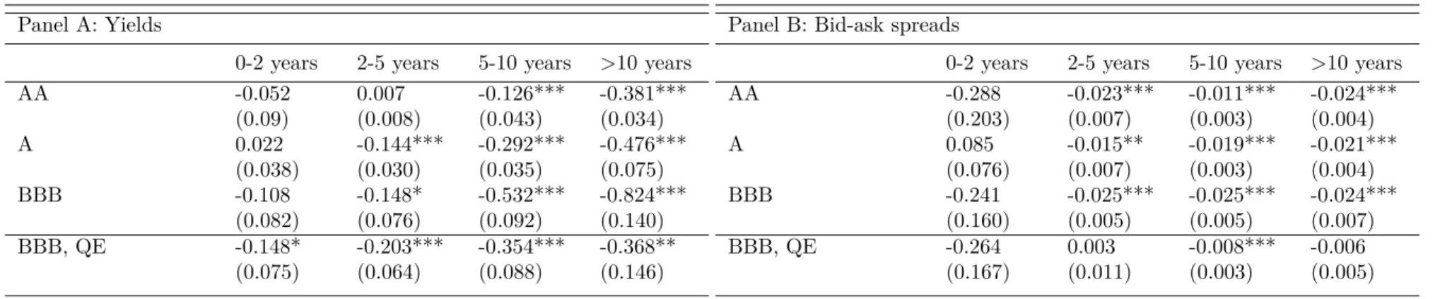
This part studies the heterogeneous QE effects for bonds with different risks. I decompose the reduction in yields into different risk premia by applying the methodology of Krishna-murthy and Vissing-Jorgensen (2011) (KVJ).7 Similar to them, I use DD regressions to isolate the duration risk channel, the default risk channel8, and the liquidity channel of QE. To dis-entangle the different risks, I split the sample of bonds into four maturity groups: 0-2 years, 2-5 years, 5-10 years and more than 10 years9, and then, within each maturity group, into three rating buckets: AA, A and BBB. All bonds within a particular maturity-rating bucket then have similar duration and default risks. To test for heterogeneous effects of QE on bonds with different risks, I run the following regression for each maturity-rating group:
yit=αi+λt+γT reat×P ost2×T reati×P ost2t+ǫit, (3) where P ost2 is a dummy equal to one after 10 March 2016 (Inter + P ost). The dependent variable is yields or bid-ask spreads.
To quantify the default risk channel of QE, I compare the yield spread of eligible versus ineligible bonds after the CSPP, within each maturity bucket. Analogously, to isolate the duration risk channel, I compare the yield spread of eligible versus ineligible bonds after QE, within each rating group. To isolate the liquidity channel, I look at the change in bid-ask spreads for eligible versus ineligible bonds after QE, within each maturity-rating bucket. The results are summarized in Table 4. Rows are different default risk groups, columns – different duration risk groups. Panel A shows the effect on yield spreads, Panel B – on bid-ask spreads. The numbers in the table are the estimates of regression (3) for bonds within a particular maturity-rating group. For example, -0.381 is the coefficient on the T reat×P ost2 dummy
for the sample of bonds rated AA, with a maturity of more than 10 years. It shows a 38.1 bps reduction in yields for QE-eligible bonds in this category, compared to ineligible bonds in the same category, after QE. In relative terms (Table A.6 in Appendix), this is a 15.25% reduction. Firm and time fixed effects are used in the regressions to account for individual and
7
I would like to thank an anonymous referee for this excellent suggestion. 8
The default risk channel is closely related to the safety premium in KVJ’s notation as the bond’s rating is used in their paper to disentangle the safety premium. For ease of notation I refer to this risk as the default risk.
9
The results are similar if I split bonds into quartiles or into 3 groups with a similar number of bonds in each: 0-2 years, 2-5 years, more than 5 years. The split of more than 10 years is to isolate the effect on the longest-maturity corporate bonds.
time-specific risks. F-statistics and number of observations are in Table A.7 in the Appendix. The point estimates in Table 4 illustrate an interesting pattern. If we fix a row, we can see that within each rating group, the statistically significant coefficients are monotonically decreasing from bonds with lower maturity to bonds with higher maturity. This result illus-trates that QE decreased yields of longer-term bonds more, compared to those of short-term bonds. The fact is consistent with the KVJ’s prediction and shows that QE had a positive effect on reducing the duration10 risk of bonds. The magnitude is the largest for lower-rated bonds close to the eligibility threshold (BBB). Moreover, if we fix a column, we can see that the significant estimates within each maturity group are also monotonically decreasing from bonds with higher ratings to bonds with lower ratings. This fact shows that QE had a posi-tive effect on reducing the default risk premium. In other words, the safety premium channel during the ECB’s QE worked in the opposite direction to the KVJ’s prediction for the Federal Reserve’s QE: the estimates in Table 4 show that the CSPP reduced yields of safer bonds less, compared to yields of riskier bonds. However, this result is not surprising given the differences between the ECB’s and the Fed’s programmes. The prediction of the KVJ study is for QE involving very safe assets, whereas the CSPP included riskier corporate bonds.
To investigate the conclusion that lower-rated bonds experienced a larger drop in yields, I restrict the sample to only treated (QE-eligible) bonds and run a DDD regression within each maturity group:
yit =αi+δ(T reati=1)t+γP ost2BBB ×T reati ×P ost2t×BBBi+ǫit (4)
Hence, the reference category in each maturity group is treated bonds with ratings higher than BBB. If the conclusion is true, the coefficients on the interaction terms should be negative. The results are presented in the last row of Panel A. As we can see, the estimates are negative and monotonically decreasing across maturity groups which shows that within each duration risk group, eligible lower-rated bonds close to the threshold experienced the largest reduction in yields.
The statistically significant bid-ask spread estimates from Panel B suggest that BBB-rated bonds also experienced the largest increase in liquidity within most maturity groups. However, the difference in liquidity for AA-rated compared to A-rated bonds is not clear. Moreover, there is no obvious pattern of liquidity improvement for bonds with different maturities within each rating group – the estimates are monotonically decreasing for A-rated bonds only. Fur-thermore, the coefficients for BBB-rated bonds within the sample of QE-eligible bonds (the last row of Panel B) show that there are minor statistically significant differences in liquidity for longer-maturity bonds. Running the DDD regression for all BBB-rated bonds (combining all maturities) shows that there are no significant liquidity changes to these bonds compared to AA-rated or A-rated bonds. The results are excluded for brevity.
In the Appendix (Table A.8), I repeat the same analysis but split the sample of bonds into 3 dimensions: duration risk, default risk, and also liquidity risk. The split in liquidity is done to isolate possible pre-existing liquidity differences for bonds with similar duration and default risks. Within each maturity-rating risk bucket bonds are further sorted into illiquid (above median ask spread) and liquid (below median ask spread) based on their
bid-10
Sorting bonds on duration instead of maturity produces almost identical results as the two are strongly correlated for the sample of bonds analyzed.
ask spreads before the QE announcement. There are fewer bonds within each maturity-rating-liquidity risk bucket and less statistically significant results but the general picture is unchanged. This fact shows that the effects in Table 4 are not due to pre-existing differences in liquidity.
The results from this subsection show that QE had heterogeneous effects on bonds with different risks. The largest impact of QE was observed for prices of bonds with higher duration and default risks. The liquidity effects, on the other hand, were only slightly different for bonds with different duration and default risks.
3.4. Discussion of the results
The substantial decrease in duration and default risks and the increase in liquidity of QE-eligible bonds documented in this section means that QE was successful in reducing the bond risk premium. This is an important result for market participants as during market crashes, this premium can become a substantial component of yields, causing a decrease in bond prices. As a consequence, banks holding risky illiquid assets may become constrained by their risk bearing capacity as in Vayanos and Vila (2009) [20], or face VaR constraints. Hence, their ability to invest in riskier instruments would be reduced and bank supply would go down. The idea of QE is then to boost economic activity by expanding the list of eligible collateral and by stimulating investors to switch to riskier investments (portfolio re-balancing channel). As the central bank steps in and implements asset purchases, it eliminates risk by reallocating the risky illiquid assets from private banks’ balance sheets to the central bank’s balance sheet, thereby relaxing the VaR constraint and decreasing the market price of risk.
The decrease in yields has two main beneficial effects. First, it allows investors to dispose of the risky QE-eligible corporate bonds by selling them to the central bank. Essentially, the increase in asset prices that QE generates is akin to a capital injection for leverage-constrained institutions. Moreover, it would allow new investors to increase their holdings of QE-eligible securities because of the reduced duration and default premiums and the fact that these securities can be sold to the central bank in the future. The results of this section show that both the price impact measures and the cost of trading of QE-eligible bonds went down indicating that investors could dispose of these bonds easier and incur lower costs in doing so. The surge in trading volume shows increased activity in QE-eligible bonds which might be related to both disposition effects (see, e.g., Koijen et al., 2017 [14]) and to new inflows into QE-eligible bonds. However, in contrast to QE-eligible bonds, the impact of QE on premiums of ineligible instruments was much weaker. Since the portfolio rebalancing channel towards riskier instruments was one of the main goals of QE, we can conclude that the ECB’s intervention achieved this goal in the subset of eligible instruments, but that the effect on ineligible bonds was less pronounced.
Second, the QE intervention would directly benefit credit-constrained corporates who could finance more cheaply on the bond market by issuing eligible bonds. The fact that the QE effects on yields were very heterogenous across different maturity-rating groups but liquidity effects were roughly similar suggests that price changes had a first order effect on corporates’ decisions to issue new bonds, whereas liquidity changes had a second order impact. The result that most of the decrease in yields within the QE-eligible segment was driven by lower-rated bonds suggests that the CSPP had a larger positive impact on riskier debt instruments and for lower-rated corporates. As we will see in the next section, these corporates made wider use of the programme.
4. Impact of QE on Corporate Debt Issuance
This section analyzes the reaction of corporates to QE. When the central bank intervenes by buying large amounts of corporate bonds, this presumably makes it easier for companies to raise capital. Essentially, the ultimate purpose of QE in this respect is to boost aggregate investment by lowering the cost of market debt issuance. The policy would allow firms that were previously unable to receive financing due to either bad quality, or asymmetric informa-tion problems, to become eligible for direct financing through the ECB. In other words, bonds issued by these firms could now be sold to the ECB, and the boost in demand by the central bank should have incentivized credit-constrained firms to start issuing more euro-denominated bonds that fulfilled the CSPP criteria after the QE announcement.
4.1. Issuance of new bonds
To detect an issuance of a new bond, I compute the age of each security on each date in the sample period. In each week, I then filter for bonds which are less than 1 week old; and this will reveal the newly issued bonds. Figure 5 shows the evolution of the number and the par of newly issued bonds in the sample period. As we can see, there was an increase both in the absolute number and in the notional amount of newly issued QE-eligible bonds after the CSPP announcement.
[Figure 5 about here]
To formally test the hypothesis that firms made use of the new cheaper funding opportunity resulting from the CSPP, I run regression (3) with the number and the par of newly issued bonds as the dependent variables. The results are presented in Table 511. As we can see from the first column of Panel A, firms issued 1.18 QE-eligible bonds more per week compared to ineligible bonds, after the CSPP. This is a 12% increase, given the mean before QE for ineligible bonds of 9.70 new bonds per week. The coefficient from column 1 of Panel B suggests that firms started issuing more QE-eligible debt after the CSPP announcement not only in number of bonds but also in notional amount. The estimate shows a 2.19 billion EUR rise of newly issued eligible debt compared to ineligible one in the post-announcement period. This is a significant increase of nearly 25%. These results suggest that corporates started to issue more QE-eligible bonds after the CSPP announcement compared to other types of debt.
However, firms issuing QE-eligible bonds might be systematically different from those issu-ing QE-ineligible bonds. To rigorously test the hypothesis that firms made use of the cheaper funding opportunity, and switched to issuing more euro-denominated QE-eligible bonds, the firm dimension is saturated in the following way. I search for firms that issue bonds in different currencies (at least one of them being the euro). There are 254 such firms (out of 1550). If there was a switch to issuing more QE-eligible debt, these firms would be more likely to issue a larger amount of their debt in euro-denominated bonds that satisfy the CSPP criteria, and less in other types of bonds. To see the cumulative effect on young bonds, I plot the total number of young bonds before the CSPP announcement, in the interim period, and following it. Figure 6 illustrates a clear increase in the number of newly issued QE-eligible bonds, which was mostly caused by issuance from BBB-rated firms. Figure 7 shows that a similar picture
11
SplittingP ost2 intoInterandP ost shows that most of the increase was coming from the interim period for all the dependent variables in the table. The results are excluded for brevity.
was observed for the par amount. Figure 8 presents the results with the euro sample split into QE-eligible and QE-ineligible bonds to show the differential effects of QE. Figure A.2 in the Appendix does the same for quarterly frequency in order to see the cumulative effect. The figures show that firms started issuing more debt in euro-denominated bonds both in absolute numbers, and in the total amount of debt. There is an increase in the par amount of QE-eligible euro bonds in the post-announcement period, but at the same time a decline in issuance of euro QE-ineligible bonds. The total amount of euro-denominated new debt in-creased slightly, and the difference with other currencies went up from the start of the interim period. These facts serve as additional evidence in favour of the hypothesis that firms issued more euro denominated QE-eligible debt as a result of the CSPP.
The DD estimates confirm these observations. The second column of Panel A in Table 5 shows that firms issuing in several currencies, switched to more QE-eligible debt. Corporates issued 1.39 QE-eligible bonds more per week after the CSPP, compared to the number of ineligible bonds. This is a 38% increase given the mean before QE for ineligible bonds of 3.70. The coefficient from column 2 of Panel B illustrates that the increase in notional value was also significant – firms issued 1.94 billion EUR more of QE-eligible debt compared to ineligible one, which is a 49% increase. Column 3 of both panels shows that corporates issued more euro-denominated bonds in general.
Next, I investigate the hypothesis that more credit-constrained firms would issue more bonds as a result of the programme. The rating of the firm is used as a proxy for credit con-straints. Although not a perfect measure, rating may serve to check which firms made wider use of the cheap financing opportunity. The logic is as follows: companies in rating categories below A that can issue eligible bonds (mostly BBB, BB) face more severe asymmetric informa-tion problems since there is a larger firm heterogeneity in these rating categories. Moreover, these companies obtain credit under less favourable conditions compared to firms rated AAA, AA or even A. The fraction of firms within each rating category and the fraction of QE-eligible bonds issued by a firm in a certain category is in Table A.11 in the Appendix. As we can see, roughly 97.71% of the QE-eligible bonds were issued by firms rated AA, A or BBB. The regression estimates from columns 4-6 in Panels A and B of Table 5 support the hypothesis that firms with lower ratings (more credit-constrained) made wider use of the cheap funding opportunity: the coefficients rise from A to BBB firms.12 BBB-rated firms issued on average 0.59 eligible bonds more each week compared to ineligible ones, after QE. In terms of par amount, they issued 0.77 billion EUR more in eligible debt. These are massive increases: 65% in number of bonds and 76% in notional terms compared to the mean of ineligible BBB-rated bonds before QE. Next, I run a DDD regression for the sample of treated bonds:
yit =αi +λt+
3
X k=1
γT reat×P ost2,k×T reati×P ost2t×Ratingk+ǫit (5) The results are even stronger. The coefficients from columns 11-13 show that the increase for AA-rated firms becomes significant and that the estimates rise from AA to A to BBB firms. Since most of the firms that can issue QE-eligible bonds are rated AA, A, or BBB, and only 2.29% are rated BB, this fact shows that there is a monotonic inverse relationship between
12
The estimates for BB-rated firms were not significant and are excluded for brevity. Running the regressions for the whole sample of firms (Table A.10 in the Appendix) produces similar results.
the rating of a firm and the amount of issued QE-eligible debt. BBB-rated firms are the ones that issued the most after the CSPP.
These results are not surprising given the evidence from Table 4. Since lower-rated eligible bonds experienced the largest drop in yields, one could expect firms with lower ratings to make wider use of the programme by issuing more bonds. This is indeed what we observe in Table 5. Another conclusion from Table 4 was that yields of longer-maturity bonds decreased the most. One could hypothesize then that firms would be more likely to issue bonds with longer maturities. To test for this, I run regression (3) for the number and the par of bonds within each maturity bucket. The coefficients from columns 7-10 in Panels A and B of Table 5 suggest that firms were more likely to issue longer-maturity bonds. The estimates for bonds with short and medium maturities (0-2 years, 2-5 years) are insignificant but the ones for longer maturities are positive and statistically significant. The coefficient for bonds with maturities of 5-10 years is the largest and shows that firms issued 0.58 (36%) eligible bonds more per week compared to ineligible ones. In terms of notional, they issued 1 billion EUR (63%) of new QE-eligible debt more each week compared to ineligible one. These facts show that the duration risk channel of QE incentivized firms to issue more bonds with longer maturities since these bonds experienced the largest drop in yields.
[Table 5 about here]
A possible caveat is that, although the regression results show that firms made use of the CSPP and issued more QE-eligible debt, it might also be that firms took even more bank credit, or used other sources of debt financing. That would cast doubt on the story developed so far. However, I rule out this possibility by looking at the ratio of bond debt outstanding to total debt for each firm. The average ratio at the end of the first quarter of 2016 was 73.41%, whereas at the end of the second quarter of 2016 it was 81.07%. This observation suggests that firms increased not only their total amount of bond debt, but also the fraction of bond debt in total liabilities. This is consistent with Gerba and Macchiarelli’s (2016) [10] findings: banks surveyed in their paper claimed that “the extra liquidity they[banks] receive has basically no impact on their decisions to grant (or not) loans”. The next step in the analysis is to see, what corporates do with the financing raised through the issuance of new QE-eligible bonds. The answer to this question is not as straightforward because there are many possible caveats and it is hard to claim that the observed effects are only due to the ECB’s intervention. I provide some analysis that attempts to answer this question, but I am aware of the different effects at play and of the possible limitations.
4.2. What do corporates do with the funds?
The results in this section are based on data from the Bureau van Dijk on firms’ dividends (D), total assets (A), fixed assets (FA), tangible fixed assets (TFA), long-term debt (LTD), R&D expenses (RD), net property, plant and equipment (PPE), working capital (WC) and cash holdings.13 Out of the 1550 distinct firms in my sample, only 417 have data on these characteristics and even less have data for the time period around the CSPP-announcement. A further limitation of the firms’ financial data is that it is only observed at quarterly frequency
13
Unfortunately, data on capital expenditures and share repurchases was available for only a tiny set of firms. There were no statistically significant effects for these indicators and the results are excluded for brevity.
compared to the weekly frequency of the Euroclear data. Another effect is that the firms in the sample are different along many dimensions (size, age, parent/daughter companies, etc.) and it is hard to argue that the only difference in observed responses is due to the issue of QE-eligible bonds. With these caveats in mind, I proceed to the empirical analysis.
I use the sample period from the first quarter of 2016 to the third quarter of 2016 and define the post period as the second and third quarters of 201614. Firms that have issued at least one QE-eligible bond are in the treatment group15. The basic regression (1) is run with firms’ financial data as the dependent variable. As Table 6 shows, most T reat×P ost
coefficients are insignificant, except the one for dividends. It might be true that firms that issue QE-eligible bonds are just larger, on average, which could partly explain the difference in the change of dividends in the post-announcement period. To address this issue, I run the regression on a sample of firms matched by total assets by splitting the firms in four quartiles based on their total assets in the first quarter of 2016. The regression coefficient (column 2) is now significant at the 1% level and shows a four times increase in dividends for firms that issued QE-eligible bonds, compared to the before-QE mean of firms not issuing QE-eligible bonds. Part of this effect, however, is due to the fact that QE-eligible firms were paying less dividends before QE compared to ineligible firms, which is governed by the negative coefficient onT reat.
[Table 6 about here]
These findings suggest that corporates used the funds attracted through the issuance of QE-eligible bonds for one-off dividend payments to current shareholders. They did not, however, change cash holdings or invest the funds in working capital, PPE or R&D. One of the goals of the QE programme was to incentivize corporates to use the attracted funds to increase investment in the real economy. To the contrary, the figures in Table 6 show that the funds were not used for this purpose in the sample of firms studied. However, these results should be interpreted with caution, given the limitations of the Bureau van Dijk data and the caveats outlined above.
Overall, the analysis in this section suggests that corporates made use of QE and issued more euro-denominated, QE-eligible debt. These results complement the literature on corpo-rate debt issuance. Consistent with the conclusions of Adrian and Shin (2012) [1], Becker and Ivashina (2014) [5] and De Fiore and Uhlig (2012) [8], I find that there is a switch to issuing more corporate debt in the aftermath of the financial crisis. The new result is that these con-clusions continue to hold even during a QE intervention and in a low-interest rate environment. Moreover, I show that more credit-constrained firms made wider use of the bond financing opportunity during a QE implementation. These new empirical findings suggest that QE was successful in providing cheap liquidity to more credit-constrained corporates, but at the same time had greater impact on firms’ dividend payments and little impact on investment.
5. Placebo tests
As a final check, this paper performs two placebo tests to verify that the sample selection of bonds in treatment and control does not mechanically produce the above results. In the
14
The results are robust to taking only the third quarter of 2016. 15
first test, the sample period is shifted backwards by 1 year to remove any effects of seasonality. A bond belongs to the treatment group if it satisfies all the QE-eligibility criteria. Similarly, the post-announcement period is defined as after 21 April 2015, as though there was a CSPP announcement on that day. Regression (1) is estimated using yields, bid-ask spreads, bilateral turnover ratio, tri-party turnover ratio, number and par of newly issued bonds as dependent variables. The results of the estimation are in Table 7, Panel A. As we can see, none of the DD estimators are statistically significant.
The second placebo test uses USD denominated bonds that satisfy all the CSPP eligibility criteria as a treatment group. These bonds share similar characteristics with the ones classified as QE-eligible earlier (maturity of less than 30 years, rating above BBB, issued by a non-credit institution, etc.) and are also similar in total numbers (479 compared to the 547 euro-denominated, QE-eligible bonds). However, the USD bonds should not be affected by the ECB’s announcement and hence should not exhibit any significant pattern around the CSPP, unless the effects I found for the QE-eligible bonds were due to some other characteristic common for all bonds satisfying the eligibility criteria. The results of regression (1) using yields, bid-ask spreads, bilateral turnover ratio, tri-party turnover ratio, number and par of newly issued bonds as dependent variables are in Table 7, Panel B. As we can see, the DD estimates are again not statistically significant.
[Table 7 about here]
The results of the second placebo test are robust to alternative specifications of the treat-ment group. I ran tests with different currencies, with a broader set of USD bonds, relaxing some of the eligibility criteria, and even with all USD denominated bonds. None of the DD estimates turned out to be statistically significant. These tests are excluded from this paper for brevity. Overall, the placebo tests rule out the possibility that the positive effects on bond yields, liquidity, and firms’ debt issuance, found in the main text, were due to seasonality, or mechanical sample selection.
6. Conclusion
This paper analyzed the impact of an unconventional QE programme on bond prices, bond liquidity and corporate debt issuance. The results show that the ECB’s CSPP decreased yields and increased liquidity in the European corporate bond market, especially in the QE-eligible segment. Yields of QE-eligible bonds decreased by 30 bps (8%) in the post-announcement period and bid-ask spreads went down by 6 bps (45%). Tri-party repo turnover increased on average by 8.15 million USD (29%) in the post-announcement period, and bilateral turnover increased by 7.05 million USD (72%). All these effects are statistically and economically significant. They were particularly pronounced for QE-eligible, lower-rated, longer-maturity bonds. These bonds experienced the largest drop in yields, which means that the ECB’s intervention had a higher positive impact on riskier debt instruments. However, there was a limited evidence for a significant shift towards ineligible, riskier bonds during the analyzed period. Since the portfolio rebalancing channel towards riskier instruments was one of the main goals of QE, I can conclude that the ECB’s intervention achieved this goal in the subset of eligible instruments, but that the effect on ineligible bonds was less pronounced. The increases in prices and liquidity show that QE was successful in reducing the bond risk premium.
of bond issuance, corporates did make use of the cheaper financing opportunity. Firms issuing in several currencies, switched to more QE-eligible debt and euro-denominated debt in general, after the CSPP announcement, compared to debt in other currencies. These effects were more pronounced for more credit-constrained firms and for longer-maturity bonds. Surprisingly, corporates used the funds attracted through the issuance of QE-eligible bonds mostly for increasing dividend payments, but did not change cash holdings or invest the funds in working capital, PPE or R&D. These results are new and show that the QE programme achieved its goal of providing cheaper credit to more credit-constrained corporates, but did not incentivize firms to increase investment. Possible extensions to this paper might include analyzing the impact of QE on firm’s default probability for firms that can issue QE-eligible debt. It would also be interesting to see, whether the ECB’s intervention actually forced investors “searching for yield” (e.g., pension funds, insurance companies) to buy more ineligible bonds in the long run.
There are many important under-researched questions about the economic effects of QE. Our knowledge of the impact of such unconventional monetary policy tools is constrained because they are relatively new and unexplored. Some critics even believe that the policy acts in the opposite direction: it provides monetary stimulus in the short run, but creates instability and exacerbates market distortions in the long run. The analysis presented here provides evidence on the relative efficiency of QE in the short term. However, as time goes by and new information becomes available, we would be in a better position to assess the impact and to fully understand the consequences of the era of unconventional monetary policy in which we are currently living.
7. Tables
Table 1: Summary statistics. The table shows summary statistics for eligible (QE) and ineligible (non-QE) bonds just before the CSPP announcement on 10 March 2016.
Age, years Maturity, years Coupon, % Par, million EUR QE non-QE QE non-QE QE non-QE QE non-QE
Mean 3.19 4.31 5.75 6.97 2.54 4.17 834.44 657.25 Standard deviation 2.67 4.17 3.00 20.64 1.48 2.37 433.20 544.13 Min 0.00 0.00 0.88 0.05 0.00 0.00 98.56 0.03 Deciles 20% 1.12 1.41 3.04 1.87 1.25 1.90 528.76 262.55 50% 2.60 2.99 5.42 4.21 2.12 4.12 728.98 549.11 70% 3.64 4.90 7.10 6.52 3.12 5.38 899.99 799.66 100% 13.79 31.38 17.72 999.62 8.12 14.00 3068.05 10255.61
Table 2: Impact of QE on bond prices and liquidity. Column 1 estimates regression (2) for bond yields (Y). Column 2 estimates the same regression with several controls (bond coupon, rating dummies, age, par amount). Column 3 estimates regression (1). Column 4 estimates regression (2) for a sample of bonds matched on par outstanding, rating and time to maturity. Column 5 estimates regression (1) with a control group consisting of all bonds that satisfy the CSPP eligibility criteria. Columns 6-7 estimate regression (1) for the bilateral turnover (BT) and the tri-party repo turnover (RT), respectively. Column 8 estimates the same specification for the bilateral market turnover ratio – BTR (here and in all subsequent regression tables measured in %) and column 9 – for the tri-party repo market turnover ratio (RTR). Column 10 estimates the same regression specification for bid-ask spreads of yields (BA). The coefficientsT reat×InterandT reat×P ostare the DD estimates of the effect of the CSPP announcement. Here and in all subsequent tables yields and bid-ask spreads are observed daily, whereas turnover and turnover ratios – weekly. Standard errors (shown in parentheses) are heteroskedasticity robust and double-clustered by firm and time (1550· 23 clusters). *,**, and *** indicate
statistical significance at the 10%, 5%, and 1% levels. Units for Y, BTR, RTR and BA: %. Units for BT, RT: million USD. Dependent variables Y Y Y Y Y BT RT BTR RTR BA (1) (2) (3) (4) (5) (6) (7) (8) (9) (10) Coupon 0.90*** (0.14) AA -2.14*** (0.39) A -2.02*** (0.45) BBB -2.07*** (0.53) BB (-0.89) (0.71) B 2.08*** (0.95) junk 19.63*** (2.85) Age -0.16*** (0.04) P ar -0.01 (0.01) T reat -2.86*** -0.61*** -5.31*** 0.20** (0.12) (0.10) (0.78) (0.10) Inter -0.24* -0.21* -0.04 -0.33*** (0.14) (0.16) (0.34) (0.02) P ost -0.37* -0.31* -1.18 -0.41*** (0.21) (0.17) (1.82) (0.03) T reat×Inter -0.22*** -0.21*** -0.22*** -0.21*** -0.13*** 2.40 1.52 0.46** 0.39** -0.02** (0.04) (0.04) (0.04) (0.03) (0.02) (1.56) (1.14) (0.21) (0.18) (0.01) T reat×P ost -0.29*** -0.29*** -0.30*** -0.28*** -0.23*** 7.05*** 8.15***1.17***1.51*** -0.06*** (0.07) (0.07) (0.07) (0.04) (0.04) (1.75) (2.25) (0.28) (0.27) (0.01) Bond Fixed Effects
and Time Dummies No No Yes No Yes Yes Yes Yes Yes Yes
Observations
(Bond-Time) 611356 611356 611356 611356 101672 115174 107875 115048 107758 611356 F-statistic 1111.33 15459.10 16523.86 360.87 368.15 125.86 76.43 81.04 52.47 38.67
Table 3: Liquidity dissipation. The table presents the estimates of regression (1) with the post-announcement period extended by four months – until 08 October 2016. Columns 1-4 present the results for the turnover measures, column 5 – for yields, and column 6 – for bid-ask spreads. Standard errors (shown in parentheses) are heteroskedasticity robust and double-clustered by firm and time. *,**, and *** indicate statistical significance at the 10%, 5%, and 1% levels. Units for Y, BTR, RTR and BA: %. Units for BT, RT: million USD.
Dependent variables BT RT BTR RTR Y BA (1) (2) (3) (4) (5) (6) T reat×Inter -1.65 -1.63 0.46** 0.38** -0.22*** -0.02** (1.84) (1.04) (0.19) (0.16) (0.04) (0.01) T reat×P ost 3.29 4.11** 0.50*** 1.30*** -0.26*** -0.07*** (2.34) (1.88) (0.15) (0.20) (0.09) (0.02) Bond Fixed Effects and Time Dummies Yes Yes Yes Yes Yes Yes Observations (Bond-Time) 195226 183295 195088 183137 1091051 1091051
Table 4: Isolating QE channels. The table presents the coefficients for theT reat×P ost2 interaction dummy in regression (3) estimated for a particular maturity-rating bucket of bonds. Panel A presents the results for yields, Panel B – for bid-ask spreads. The last row in each panel estimates DDD regression (4) only for the sample of treated bonds. Each regression has firm and time fixed effects. Standard errors (shown in parentheses) are heteroskedasticity robust and double-clustered by firm and time. *,**, and *** indicate statistical significance at the 10%, 5%, and 1% levels. Units for all estimates: %.
Panel A: Yields
0-2 years 2-5 years 5-10 years >10 years
AA -0.052 0.007 -0.126*** -0.381*** (0.09) (0.008) (0.043) (0.034) A 0.022 -0.144*** -0.292*** -0.476*** (0.038) (0.030) (0.035) (0.075) BBB -0.108 -0.148* -0.532*** -0.824*** (0.082) (0.076) (0.092) (0.140) BBB, QE -0.148* -0.203*** -0.354*** -0.368** (0.075) (0.064) (0.088) (0.146)
Panel B: Bid-ask spreads
0-2 years 2-5 years 5-10 years >10 years AA -0.288 -0.023*** -0.011*** -0.024*** (0.203) (0.007) (0.003) (0.004) A 0.085 -0.015** -0.019*** -0.021*** (0.076) (0.007) (0.003) (0.004) BBB -0.241 -0.025*** -0.025*** -0.024*** (0.160) (0.005) (0.005) (0.007) BBB, QE -0.264 0.003 -0.008*** -0.006 (0.167) (0.011) (0.003) (0.005) 23