Efficient Market Making via Convex Optimization, and a Connection to Online Learning

Efficient Market Making via Convex Optimization, and a Connection

to Online Learning

Jacob Abernethy, University of Pennsylvania

Yiling Chen, Harvard University

Jennifer Wortman Vaughan, University of California, Los Angeles

We propose a general framework for the design of securities markets over combinatorial or infinite state or outcome spaces. The framework enables the design of computationally efficient markets tailored to an arbitrary, yet relatively small, space of securities with bounded payoff. We prove that any market satisfying a set of intuitive conditions must price securities via a convex cost function, which is constructed via conju-gate duality. Rather than deal with an exponentially large or infinite outcome space directly, our framework only requires optimization over a convex hull. By reducing the problem of automated market making to convex optimization, where many efficient algorithms exist, we arrive at a range of new polynomial-time pricing mechanisms for various problems. We demonstrate the advantages of this framework with the de-sign of some particular markets. We also show that by relaxing the convex hull we can gain computational tractability without compromising the market institution’s bounded budget. Although our framework was designed with the goal of deriving efficient automated market makers for markets with very large outcome spaces, this framework also provides new insights into the relationship between market design and machine learning, and into the complete market setting. Using our framework, we illustrate the mathematical paral-lels between cost function based markets and online learning and establish a correspondence between cost function based markets and market scoring rules for complete markets.

Categories and Subject Descriptors: F.0 [Theory of Computation]: General; J.4 [Computer Applica-tions]: Social and Behavioral Sciences

General Terms: Algorithms, Economics, Theory

Additional Key Words and Phrases: Market design, securities market, prediction market, automated market maker, convex analysis, online linear optimization

ACM Reference Format:

Abernethy, J., Chen, Y., Vaughan, J. W. 2012. Efficient Market Making via Convex Optimization, and a Connection to Online Learning. ACM TEAC 1, 1, Article X ( 2012), 38 pages.

DOI=10.1145/0000000.0000000 http://doi.acm.org/10.1145/0000000.0000000

Parts of this research initially appeared in Chen and Vaughan [2010] and Abernethy et al. [2011].

This work is supported NSF grants CCF-0953516, CCF-0915016, IIS-1054911, and DMS-070706, DARPA grant FA8750-05-2-0249, and a Yahoo! PhD Fellowship, and is based on work that was supported by NSF under CNS-0937060 to the CRA for the CIFellows Project. Any opinions, findings, conclusions, or recom-mendations expressed in this material are those of the authors alone. The authors are grateful to David Pennock for useful discussions about this work and Xiaolong Li and Michael Ruberry for comments on an earlier draft.

Author’s addresses: J. Abernethy, Computer and Information Science Department, University of Pennsyl-vania; Y. Chen, School of Engineering and Applied Sciences, Harvard University; J. W. Vaughan, Computer Science Department, University of California, Los Angeles.

Permission to make digital or hard copies of part or all of this work for personal or classroom use is granted without fee provided that copies are not made or distributed for profit or commercial advantage and that copies show this notice on the first page or initial screen of a display along with the full citation. Copyrights for components of this work owned by others than ACM must be honored. Abstracting with credit is per-mitted. To copy otherwise, to republish, to post on servers, to redistribute to lists, or to use any component of this work in other works requires prior specific permission and/or a fee. Permissions may be requested from Publications Dept., ACM, Inc., 2 Penn Plaza, Suite 701, New York, NY 10121-0701 USA, fax+1 (212) 869-0481, or [email protected].

c

2012 ACM 0000-0000/2012/-ARTX $15.00

1. INTRODUCTION

Securities marketsplay a fundamental role in economics and finance. A securities mar-ket offers a set ofcontingent securitieswhose payoffs depend on the future state of the world. For example, an Arrow-Debreu security pays $1 if a particular state of the world is reached and $0 otherwise [Arrow 1964; 1970]. Consider an Arrow-Debreu security that will pay off in the event that a category 4 or higher hurricane passes through Florida in 2012. A Florida resident who worries about his home being damaged might buy this security as a form of insurance to hedge his risk; if there is a hurricane pow-erful enough to damage his home, he will be compensated. Additionally, a risk-neutral trader who has reason to believe that the probability of a category 4 or higher hurri-cane landing in Florida in 2012 ispshould be willing to buy this security at any price belowpor (short) sell it at any price abovepto capitalize his information. For this rea-son, the market price of the security can be viewed as the traders’ collective estimate of how likely it is that a powerful hurricane will occur. Securities markets thus have dual functions:risk allocationandinformation aggregation.

Insurance contracts, options, futures, and many other financial derivatives are ex-amples of contingent securities. A securities market primarily focused on information aggregation is often referred to as a prediction market. The forecasts of prediction markets have proved to be accurate in a variety of domains [Ledyard et al. 2009; Berg et al. 2001; Wolfers and Zitzewitz 2004]. While our work builds on ideas from predic-tion market design [Chen and Vaughan 2010; Othman et al. 2010; Agrawal et al. 2011], our framework can be applied to any contingent securities.

A securities market is said to be completeif it offers at least |O|linearly indepen-dent securities over a setOof mutually exclusive and exhaustive states of the world, which we refer to asoutcomes[Arrow 1964; 1970; Mas-Colell et al. 1995]. For example, a prediction market withnArrow-Debreu securities fornoutcomes is complete. In a complete securities market without transaction fees, a trader may bet on any combi-nation of the securities, allowing him to hedge any possible risk he may have. It is generally assumed that the trader mayshort sella security, betting against the given outcome; in a market with short selling, thenth security is not strictly necessary, as a trader can substitute the purchase of this security by short selling all others. Further-more, traders can change the market prices to reflect any valid probability distribution over the outcome space, allowing them to reveal any belief. Completeness therefore provides expressiveness for both risk allocation and information aggregation.

Unfortunately, completeness is not always achievable. In many real-world settings, the outcome space is exponentially large or even infinite. For instance, a competitive race betweennathletes results in an outcome space ofn!rank orders, while the future price of a stock has an infinite outcome space, namelyR≥0. In such situations operating

a complete securities market is not practical for two reasons: (a) humans are notori-ously bad at estimating small probabilities and (b) it is computationally intractable to manage such a large set of securities. Instead, it is natural to offer a smaller set of structured securities. For example, rather than offer a security corresponding to each rank ordering, in pair bettinga market institution offers securities of the form “$1 if candidate A beats candidate B” [Chen et al. 2007a; Chen et al. 2008a]. There has been a surge of recent research examining the tractability of running standard prediction market mechanisms (such as the popular Logarithmic Market Scoring Rule (LMSR) market maker [Hanson 2003]) over combinatorial outcome spaces by limiting the space of available securities [Pennock and Sami 2007]. While this line of research has led to a few positive results [Chen et al. 2007b; Chen et al. 2008b; Guo and Pennock 2009; Agrawal et al. 2008], it has led more often to hardness results [Chen et al. 2007b; Chen

et al. 2008a] or to markets with undesirable properties such as unbounded loss of the market institution [Gao et al. 2009].

In this paper, we propose a general framework to design automated market mak-ersfor securities markets. An automated market maker is a market institution that adaptively sets prices for each security and is always willing to accept trades at these prices. Unlike previous research aimed at finding a space of securities that can be efficiently priced using an existing market maker like the LMSR, we start with an ar-bitrary space of securities and design anewmarket maker tailored to this space. Our framework is therefore very general and includes existing market makers for complete markets, such as the LMSR and Quad-SCPM [Agrawal et al. 2011], as special cases.

We take an axiomatic approach. Given a relatively small space of securities with bounded payoff, we define a set of intuitive conditions that a reasonable market maker should satisfy. We prove that a market maker satisfying these conditions must price securities via a convex potential function (the cost function), and that the space of reachable security prices must be precisely the convex hull of the payoff vectors for each outcome (that is, the set of vectors, one per outcome, denoting the payoff for each security if that outcome occurs). We then incorporate ideas from online convex opti-mization [Hazan 2009; Rakhlin 2009] to define a convex cost function in terms of an optimization over this convex hull; the vector of prices is chosen as the optimizer of this convex objective. With this framework, instead of dealing with the exponentially large or infinite outcome space, we only need to deal with the lower-dimensional convex hull. The problem of automated market making is reduced to the problem of convex optimization, for which we have many efficient techniques to leverage.

To demonstrate the advantages of our framework, we provide two new computation-ally efficient markets. The first market can efficiently price subset bets on permuta-tions, which are known to be #P-hard to price using the LMSR [Chen et al. 2008a]. The second market can be used to price bets on the landing location of an object on a sphere. For situations where the convex hull cannot be efficiently represented, we show that we can relax the convex hull to gain computational tractability without compromising the market maker’s bounded budget. This allows us to provide a com-putationally efficient market maker for the aforementioned pair betting, which is also known to be #P-hard to price using the LMSR [Chen et al. 2008a].

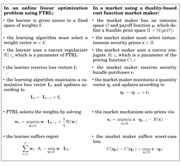
Although our framework was designed with the goal of deriving novel, efficient au-tomated market makers for markets with very large outcome spaces, this framework also provides new insights into the relationship between market design and machine learning, and into the complete market setting. With our framework, we illustrate the mathematical parallels between cost function based markets and online learning, and establish a correspondence between cost function based markets and market scoring rules for complete markets.

Roadmap of the paper: The rest of the paper is organized as follows. We begin in Section 2 with a review of the relevant literature on automated market makers and prediction market design. In Section 3 we describe the problem of market design for large outcome spaces, discuss the difficulties inherent to this problem, and introduce our axiomatic approach. In Section 4 we give a detailed framework for constructing pricing mechanisms based on convex optimization and conjugate duality. We give a couple of examples of efficient duality-based cost function market makers in Section 5. In Section 6 we consider the computational issues associated with our framework, and show how the proposed convex optimization problem can be relaxed to gain tractability without increasing the worst-case loss of the market maker. We illustrate the mathe-matical parallels between our framework and online learning in Section 7. Finally, in

Section 8, we describe how our framework can be used to establish a correspondence between cost function based markets and market scoring rules for complete markets.

2. BACKGROUND AND RELATED WORK

Automated market makers for complete markets are well studied in both economics and finance. Our work builds on the literature on cost function based markets [Hanson 2003; 2007; Chen and Pennock 2007]. A simple cost function based market maker offers |O| Arrow-Debreu securities, each corresponding to a potential outcome. The market maker determines how much each security should cost using a differentiable

cost function,C:R|O|→R, which is simply a potential function specifying the amount

of money currently wagered in the market as a function of the number of shares of each security that have been purchased. If qo is the number of shares of security o

currently held by traders, and a trader would like to purchase a bundle of ro shares

for each securityo∈ O(where eachrocould be positive, representing a purchase, zero,

or even negative, representing a sale), the trader must pay C(q+r)−C(q) to the market maker. The instantaneous price of securityo(that is, the price per share of an infinitesimal portion of a security) is then∂C(q)/∂qo, and is denotedpo(q).

One example of a cost function based market that has received considerable atten-tion is Hanson’s Logarithmic Market Scoring Rule (LMSR) [Hanson 2003; 2007; Chen and Pennock 2007]. The cost function of the LMSR is

C(q) =blogX

o∈O

eqo/b_{, (1)}

whereb >0is a parameter of the market controlling the rate at which prices change. The corresponding price function for each securityois

po(q) = ∂C(q) ∂qo = e qo/b P o0_∈Oeqo0/b . (2)

It is well known that the monetary loss of an automated market maker using the LMSR is upperbounded byblog|O|. Additionally, the LMSR satisfies several other de-sirable properties, which are discussed in more detail in Section 3.1.

When|O|is large or infinite, calculating the cost of a purchase becomes intractable in general. Recent research on automated market makers for large outcome spaces has focused on restricting the allowable securities over a combinatorial outcome space and examining whether the LMSR prices can be computed efficiently in the restricted space. If the outcome space contains n! rank orders of ncompeting candidates, it is #P-hard to price pair bets(securities of the form “$1 if and only if candidate A beats candidate B”) or subset bets (for example, “$1 if one of the candidates in subset C finishes at position k”) using the LMSR on the full set of permutations [Chen et al. 2008a]. If the outcome space contains2n_{Boolean values ofnbinary base events, it is}

#P-hard to price securities on conjunctions of any two base events (for example, “$1 if and only if a Democrat wins Florida and Ohio”) using the LMSR [Chen et al. 2008a]. This line of research has led to some positive results when the uncertain event enforces particular structure on the outcome space. In particular, for a single-elimination tour-nament of n teams, securities such as “$1 if and only if team A wins a kth round game” and “$1 if and only if team A beats team B given they face off ” can be priced efficiently using the LMSR [Chen et al. 2008b]. The tractability of these securities is due to a structure-preserving property — the market probability can be represented by a Bayesian network and price updating does not change the structure of the net-work. Pennock and Xia [2011] significantly generalized this result and characterize all structure-preserving securities. For a taxonomy tree on some statistic where the value

of the statistic of a parent node is the sum of those of its children, securities such as “$1 if and only if the value of the statistic at node A belongs to[x, y]” can be priced efficiently using the LMSR [Guo and Pennock 2009].

One approach to combat the computational intractability of pricing over combina-torial spaces is to approximate the market prices using sampling techniques. Yahoo!’s Predictalot,1_{a play-money combinatorial prediction market for the NCAA Men’s}

Bas-ketball playoff, allows traders to bet on almost any combination of the 263 _outcomes

of the tournament. Predictalot is based on the LMSR. Instead of calculating the ex-act prices for securities, it uses importance sampling to approximate the prices. Xia and Pennock [2011] devised a Monte-Carlo algorithm that can efficiently compute the price of any security in disjunctive or conjunctive normal form with guaranteed er-ror bounds. However, using sampling techniques brings a new problem to pricing. The sampling algorithm in general won’t give the same prices if quoted twice, even if the market status remains the same. Because of this, traders can exploit the market to make a profit, which increases the loss of the market maker.

In this paper, we take a drastically different approach to combinatorial market design. Instead of searching for supportable spaces of securities for existing market makers, we design new market makers tailored to any security space of interest and with desirable theoretical properties. Additionally, rather than requiring that securi-ties have a fixed (e.g., $1) payoff when the underlying event happens, we allow more general contingent securities with arbitrary, efficiently computable and bounded pay-offs.

Our approach makes use of powerful techniques from convex optimization. Agrawal et al. [2011] and Peters et al. [2007] also use convex optimization for automated market making. One major difference is that they only consider complete markets, while we consider markets with an arbitrary set of securities. They consider the setting in which traders submit limit orders, and formulate a convex optimization problem that can be solved by the market institution in order to decide what quantity of orders to accept. While formulating the problem in terms of limit orders leads to a syntactically different problem, their mechanisms can be turned into equivalent cost function based market makers. Agrawal et al. [2011] show that their mechanisms can be formulated as a risk minimization problem with an associated penalty function. Mathematically the penalty function plays a similar role as the conjugate function R in our framework, but they do not explicitly make a connection with conjugate duality.

This paper focuses on cost function based market makers. It is worth noting that there are other market mechanisms, with different properties, designed for securities markets. For complete markets, Dynamic Parimutuel Markets [Pennock 2004; Man-gold et al. 2005] also use a cost function to price securities, however the securities are parimutuel bets whose future payoff is not fixed a priori, but depends on the market activities. Brahma et al. [2010] and Das and Magdon-Ismail [2008] design Bayesian learning market makers that maintain a belief distribution and update it based on the traders’ behavior. Call markets have been studied to trade securities over com-binatorial spaces. In a call market, participants submit limit orders and the market institution determines what orders to accept or reject. Researchers have studied the computational complexity of operating call markets for both permutation [Chen et al. 2007b; Agrawal et al. 2008; Ghodsi et al. 2008] and Boolean [Fortnow et al. 2004] com-binatorics.

Related work on online learning and related work on market scoring rules are dis-cussed in Sections 7 and 8 respectively.

3. AN AXIOMATIC APPROACH TO MARKET DESIGN

In this work, we are primarily interested in a market-design scenario in which the outcome spaceOis exponentially large, or even infinite, making it infeasible to run a complete market; not only is it generally intractable for the market maker to price an exponential number of securities, but it is notoriously difficult for human traders to reason about the probabilities of so many individually unlikely outcomes. To address both of these problems, we restrict the market maker to offer a menu of only K se-curities for some reasonably-sizedK. These securities will be designed by the market maker and one can interpret each security as corresponding to some “interesting” or “useful” query that we might like to make about the future outcome. For example, if a set of players compete in a tournament, the market maker can offer a security for every question of the form “does playerX survive beyond roundY?”

We assume that the payoff of each security, clearly depending on the future outcome o, can be described by an arbitrary but efficiently-computable functionρ:O →RK≥0; if a

trader purchases a share of securityiand the true outcome iso, then the trader is paid ρi(o). We call such a security spacecomplex. The complete security space is a special

case of a complex security space in which K =|O|and for eachi ∈ {1,· · ·, K}, ρi(o)

equals 1 ifois theith outcome and0otherwise. The markets we design enable traders to purchase arbitrarysecurity bundlesr∈RK. A negative element ofrencodes a sale

of such a security. The payoff forrupon outcomeois exactlyρ(o)·r, whereρ(o)denotes the vector of payoffs for each security for outcomeo. Let us defineρ(O) :={ρ(o)|o∈ O}.

It will be assumed, throughout the paper, thatρ(O)is closed and bounded.

The first step in the design of automated market makers for complex security spaces is to determine an appropriate set of properties that we would like such market makers to satisfy. To build intuition about which properties might be desirable, we first step back and consider what it is that makes a market maker like the LMSR a good choice for complete markets.

3.1. What Makes A Market Maker Reasonable?

Consider the cost function associated with the Logarithmic Market Scoring Rule (Equation 1) and the corresponding instantaneous price functions (Equation 2). This cost function and the resulting market satisfy several natural properties that make the LMSR a “reasonable” choice:

(1) The cost function is differentiable everywhere. As a result, an instantaneous price po(q) = ∂C(q)/∂qo can always be obtained for the security associated with any

outcomeo, regardless of the current quantity vectorq.

(2) The market incorporates information from the traders, in the sense that the pur-chase of a security corresponding to outcomeocausespoto increase.

(3) The market does not provide explicit opportunities for arbitrage. Since instanta-neous prices are never negative, traders are never paid to obtain securities. Ad-ditionally, the sum of the instantaneous prices of the securities is always 1. If the prices summed to something less than (respectively, greater than) 1, a trader could purchase (respectively, short sell) small equal quantities of each security for a guaranteed profit. This is prevented. In addition to preventing arbitrage, these properties also ensure that prices can be interpreted naturally as probabilities, representing the market’s current estimate of the distribution over outcomes.

(4) The market isexpressivein the sense that a trader with sufficient funds can always set the market prices to reflect his beliefs about the probability of each outcome.2

As described in Section 2, previous research on cost function based markets for com-binatorial outcome spaces has focused on developing algorithms to efficiently imple-ment or approximate LMSR pricing [Chen et al. 2008a; Chen et al. 2008b; Guo and Pennock 2009]. Because of this, there has been no need to explicitly extend these prop-erties to complex markets; the propprop-erties hold automatically for any implementation of the LMSR. This is no longer the case when our goal is to design new markets tailored to custom sets of securities.

To gain intuition about what makes an arbitrary complex market “reasonable,” let us begin by considering the example of pair betting [Chen et al. 2007a; Chen et al. 2008a]. Suppose our outcome space consists of rankings of a set ofncompetitors, such asnhorses in a race. The outcome of such a race is a permutationπ: [n]→[n], where [n]denotes the set{1,· · · , n}, andπ(i)is the final position ofi, withπ(i) = 1being best. A typical market for this setting might offernsecurities, with theith security paying off $1 π(i) = 1and $0 otherwise. Additionally, there might be separate, independent

markets allowing bets on horses to place (come in first or second) or show (come in first, second, or third). However, running independent markets for sets of outcomes with clear correlations is wasteful in that information revealed in one market does not automatically propagate to the others. Instead, suppose that we would like to define a set of securities that allow traders to make arbitrary pair bets; that is, for every i, j, a trader can purchase a security which pays out $1 wheneverπ(i) < π(j). What properties would make a market for pair bets reasonable?

The first two properties described above have straight-forward interpretations in this setting. We would still like the instantaneous price of each security to be well-defined at all times; intuitively, the instantaneous price of the security forπ(i)< π(j) should represent the traders’ collective belief about the probability that horseifinishes ahead of horse j. Call this price pi,j. We would still like the market to incorporate

information, in the sense that buying the security corresponding toπ(i)< π(j)should never cause the pricepi,jto drop.

The remaining two properties are more tricky to quantify. Intuitively, these proper-ties require us to define a set of constraints over the prices achievable in the market (to prevent arbitrage), and to ensure that any prices reflecting consistent beliefs about the distribution over outcomes can be achieved (for expressiveness). One can come up with various logical constraints that prices should satisfy. For example,pi,j must be

nonnegative at all times for alliandj, andpi,j+pj,imust always equal 1 since exactly

one of the two securities corresponding toπ(i)< π(j)andπ(j)< π(i)respectively will pay out $1. Similar reasoning gives us the additional constraint that for alli, j, and k, pi,j +pj,k+pk,i must be at least 1 and no more than 2. But are these constraints

enough to prevent arbitrage? Are they too strong to allow the expression of arbitrary consistent beliefs?

In general, this type of ad hoc reasoning can lead us to many apparently reasonable constraints, but does not yield an algorithm to determine whether or not we have generated the full set of constraints necessary to prevent arbitrage, and cannot be applied easily to more complicated security spaces. We address this problem in the next section. We start by formalizing the desirable market properties described above in the context of complex markets. We then provide a precise mathematical characterization of all cost functions that satisfy these properties.

3.2. An Axiomatic Characterization of Complex Markets

We are now ready to formalize a set of conditions or axioms that one might expect a market to satisfy, and show that these conditions lead to some natural mathematical restrictions on the costs of security bundles. (We consider relaxations of these condi-tions in Section 6.) We do not presuppose a cost function based market. However, we show that the use of a convex cost function isnecessarygiven the assumption of path independence on the security purchases.

3.2.1. Path Independence and the Use of Cost Functions. Imagine a sequence of traders entering the marketplace and purchasing security bundles. Letr1,r2,r3, . . .be the se-quence of security bundles purchased. Aftert−1such purchases, thet-th trader should be able to enter the marketplace and query the market maker for the cost of arbitrary bundles. The market maker must be able to furnish a cost, denotedCost(r|r1, . . . ,rt−1),

for any bundlergiven a previous trade sequencer1, . . . ,rt−1. If the trader chooses to

purchasert at a cost ofCost(rt|r1, . . . ,rt−1), the market maker may update the costs

of each bundle accordingly. Our first condition requires that the cost of acquiring a bundlermust be the same regardless of how the trader splits up the purchase.

CONDITION1 (PATHINDEPENDENCE). For anyr,r0, andr00such thatr=r0+r00, for anyr1, . . . ,rt,

Cost(r|r1, . . . ,rt) =Cost(r0|r1, . . . ,rt) +Cost(r00|r1, . . . ,rt,r0).

Path independence helps to reduce both arbitrage opportunities and the strategic play of traders, as traders need not reason about the optimal path leading to some target position. However, it is worth pointing out that there are interesting markets that do not satisfy this condition, such as the continuous double auction and the mar-ket maker for continuous double auctions considered by Brahma et al. [2010] and Das and Magdon-Ismail [2008]. These markets do not fall into our framework and deserve separate treatment.

It turns out that the path independence alone implies that prices can be represented by a cost functionC, as illustrated in the following theorem.

THEOREM 3.1. Under Condition 1, there exists a cost functionC : RK → R such that we may always write

Cost(rt|r1, . . . ,rt−1) =C(r1+. . .+rt−1+rt)−C(r1+. . .+rt−1).

PROOF. Let C(q) := Cost(q|∅). Clearly C(0) = Cost(0|∅) = 0. We will show, via induction ont, that for anytand any bundle sequencer1, . . . ,rt,

Cost(rt|r1, . . . ,rt−1) =C(r1+. . .+rt−1+rt)−C(r1+. . .+rt−1). (3)

When t = 1, this holds trivially. Assume that Equation 3 holds for all bundle se-quences of any lengtht≤T. By Condition 1,

Cost(rT+1|r1, . . . ,rT) = Cost(rT+1+rT|r1, . . . ,rT−1)−Cost(rT|r1, . . . ,rT−1) = C rT+1+rT + T−1 X t=1 rt ! −C T−1 X t=1 rt ! − C rT+ T−1 X t=1 rt ! −C T−1 X t=1 rt !! = C T+1 X t=1 rt ! −C T X t=1 rt ! ,

and we see that Equation 3 holds fort=T+ 1too.

With this theorem in mind, we drop the cumbersomeCost(r|r1, . . . ,rt)notation from now on, and write the cost of a bundlerasC(q+r)−C(q), whereq=r1+. . .+rtis the vector of previous purchases.

3.2.2. Formalizing the Properties of a Reasonable Market.Recall that one of the func-tions of a securities market is to aggregate traders’ beliefs into an accurate predic-tion. Each trader may have his own (potentially secret) information about the fu-ture, which we represent as a distribution p ∈ ∆|O| over the outcome space, where

∆n ={x ∈ Rn≥0 :

Pn

i=1xi = 1}, then-simplex. The pricing mechanism should

there-fore incentivize the traders to revealp, but simultaneously avoid providing arbitrage opportunities. Towards this goal, we now revisit the relevant properties of the LMSR discussed in Section 3.2, and show how the ideas behind each of these properties can be extended to the complex market setting, yielding four additional conditions on our pricing mechanism.

The first condition ensures that the gradient ofC,∇C(q), is always well-defined. If we imagine that a trader can buy or sell an arbitrarily small bundle, we would like the cost of buying and selling an infinitesimal quantity of any particular bundle to be the same. If∇C(q)is well-defined, it can be interpreted as a vector of instantaneous prices for each security, with ∂C(q)/∂qi representing the price per share of an infinitesimal

amount of securityi. Additionally, we can interpret ∇C(q)as the traders’ current es-timates of the expected payoff of each security, in the same way that∂C(q)/∂qo was

interpreted as the probability of outcome o when considering the complete security space.

CONDITION2 (EXISTENCE OFINSTANTANEOUSPRICES). C is continuous and

differentiable everywhere onRK.

The next condition encompasses the idea that the market should react to trades in a sensible way in order to incorporate the private information of the traders. In par-ticular, it says that the purchase of a security bundlershould never cause the market to lower the price ofr. This condition is closely related to incentive compatibility for a myopic trader. It is equivalent to requiring that a trader with a distributionp∈∆|O|

can never find it profitable (in expectation) to buy a bundlerand at the same time find it profitable to buy the bundle−r. In other words, there can not be more than one way to express one’s information.

CONDITION3 (INFORMATIONINCORPORATION). For any q and r ∈ RK, C(q+

2r)−C(q+r)≥C(q+r)−C(q).

The no arbitrage condition states that it is never possible for a trader to purchase a security bundle rand receive a positive profit regardless of the outcome. Without this property, the market maker would occasionally offer traders a chance to obtain a guaranteed profit, which is clearly suboptimal in terms of the market maker’s loss. However, we do consider the relaxation of this property in Section 6.

CONDITION4 (NOARBITRAGE). For allq,r∈RK, there exists ano∈ Osuch that

C(q+r)−C(q)≥r·ρ(o).

Finally, the expressiveness condition specifies that any trader can set the market prices to reflect his beliefs, within any error, about the expected payoffs of each se-curity if arbitrarily small portions of shares may be purchased. The approximation factor is necessary because the trader’s beliefs may only be expressible in the limit;

note that the LMSR does not allow a trader to express the belief that an outcome will occur with probability1except in the limit.

CONDITION5 (EXPRESSIVENESS). For any p ∈ ∆|O|, we write xp := Eo∼p[ρ(o)]. Then for anyp∈∆|O|and any >0there is someq∈RK for whichk∇C(q)−xpk< .

Having formalized our set of conditions, we must now address the question of how to determine whether or not these conditions are satisfied for a particular cost functionC. The following theorem precisely characterizes the set of all cost functions that satisfy these conditions. The statement and proof require the use of a few pieces of terminology from convex optimization, which will be our main tool for designing cost functions that satisfy Conditions 2-5; for more on why this is necessary, see the note in Section 4. In particular, therelative boundaryof a convex setSis its boundary in the “ambient” dimension of S. For example, if we consider the n-dimensional probability simplex ∆n := {x ∈ Rn : Pixi = 1,∀i xi ≥ 0}, then the relative boundary of ∆n is the set

{x ∈ ∆n : xi = 0for somei}. We use relint(S) to refer to the relative interior of a

convex setS, which is the setS minus all of the points on the relative boundary. The interior of a square in 3-dimensional space is empty, but the relative interior is not. We will use closure(S)to refer to the closure of S, the smallest closed set containing all of the limit points ofS. For any subsetS ofRd, letH(S)denote the convex hull of

S. An important object, which we will use throughout the paper, isH(ρ(O))the convex hull of the set of outcome payoffs. (Recall that ρ(O) := {ρ(o)|o ∈ O}.) As we have assumed that ρ(O) is a closed set, it follows easily that H(ρ(O)) is also closed, and hence closure(H(ρ(O))) =H(ρ(O)).

THEOREM 3.2. Under Conditions 2-5,Cmust be convex with

closure({∇C(q) :q∈RK}) =H(ρ(O)). (4) Moreover, any convex differentiable functionC:_RK _→

Rrespecting(4)must also satisfy Conditions 2-5.

PROOF. We begin with the first direction. Take anyCsatisfying Conditions 2-5. We first establish thatCis convex everywhere. AssumeCis non-convex somewhere. Then there must exist some qand rsuch thatC(q)> (1/2)C(q+r) + (1/2)C(q−r). This meansC(q+r)−C(q)< C(q)−C(q−r), which contradicts Condition 3, soCmust be convex.

To prove the equality, we will establish containment in both directions. We first prove that {∇C(q) : q ∈ RK} ⊂ H(ρ(O)), from which it follows that closure({∇C(q) : q ∈ RK})⊆ H(ρ(O))becauseH(ρ(O))is already closed by assumption. Notice that

Condi-tion 2 trivially guarantees that∇C(q)is well-defined for anyq. Towards a contradic-tion, let us assume there exists someq0 for which∇C(q0)∈ H(ρ(O))/ . Because the hull is a convex set, this can be reformulated in the following way: There must exist some halfspace, defined by a normal vectorr, that separates∇C(q0)from every member of ρ(O). More precisely

∇C(q0)∈ H(ρ(O))/ ⇐⇒ ∃r∀o∈ O:∇C(q0)·r<ρ(o)·r.

The strict inequality in this equation is due to the assumption thatH(ρ(O))is a closed convex set. On the other hand, letting q := q0 −r, we see by convexity of C that C(q+r)−C(q)≤ ∇C(q0)·r. Combining these last two inequalities, we see that the price of bundlerpurchased with historyqis always smaller than the payoff foranyoutcome. This implies that there exists some arbitrage opportunity, contradicting Condition 4.

We now show thatH(ρ(O))⊆closure({∇C(q) :q∈ RK}). The statement of

of the set{∇C(q) :q∈RK}. But then we are done, as the closure(S)is defined as the

Sincluding all of its limit points.

We now prove the final statement, which is that (4) is also sufficient to achieve Condi-tions 2-5. Take some convex differentiableC:RK →Rfor which (4) is true. Condition 2

follows by definition. As previously argued, Condition 3 is equivalent to the convexity ofC. Condition 5 is equivalent to the statement thatH(ρ(O))⊆closure({∇C(q) :q∈

RK}). Finally, to establish Condition 4, we have to reverse our previous argument.

The existence of an arbitrage opportunity means that there exist someq,rsuch that C(q+r)−C(q) < ρ(o)·r for each o ∈ O. Using convexity of C, we also have that ∇C(q)·r≤C(q+r)−C(q). Combining gives us that∇C(q)·r≤ρ(o)·rfor allo∈ O, but this last statement is equivalent to the statement that∇C(q)∈ H(ρ(O))/ . This is a contradiction and thus Condition 4 is satisfied.

What we have arrived at from the set of proposed conditions is that (a) a pricing mechanism can always be described precisely in terms of a convex cost function C and (b) the set of reachable prices of a mechanism, that is the set{∇C(q) : q∈RK},

must be identically the convex hull of the payoff vectors for each outcome H(ρ(O)) except possibly differing at the relative boundary of H(ρ(O)). For complete markets, this would imply that the set of achievable prices should be the convex hull of the nstandard basis vectors. Indeed, this comports exactly with the natural assumption that the vector of security prices in complete markets should represent a probability distribution, or equivalently that it should lie in then-simplex [Agrawal et al. 2011].

4. DESIGNING THE COST FUNCTION VIA CONJUGATE DUALITY

The natural conditions we introduced above imply that to design a market for a set of K securities with payoffs specified by an arbitrary payoff function ρ : O → RK≥0,

we should use a cost function based market with a convex, differentiable cost function such that closure({∇C(q) :q∈RK}) =H(ρ(O)). We now provide a general technique

that can be used to design and compare properties of cost functions that satisfy these criteria. Our proposed framework uses the notionconjugate dualityto construct cost functions. The aim here is to simplify the task of designing a functionCwhich satisfies Conditions 2-5. We refer to any market mechanism belonging to our framework as a

Duality-based Cost Function Market Maker.

Duality-based Cost Function Market Maker Input:Outcome spaceO

Input:Ksecurities specified by a payoff functionρ:O →RK≥0 Input:Convex compact price spaceΠ(typicallyΠ≡ H(ρ(O)))

Input:Strictly convexRwith relint(Π)⊆dom(R)

Output:Market mechanism specified by the cost functionC:RK →Rwith

C(q) := sup

x∈relint(Π)

x·q−R(x)

To understand this framework, we begin by reviewing the definition of a convex conjugate. Here and throughout the paper we use the notation dom(f)to refer to the domain of a functionf, i.e., where it is defined and finite valued.

Definition4.1 (Rockafellar [1970], Section 12). For any convex functionf :RK →

[−∞,∞], theconvex conjugatef∗off is defined as f∗(z) := sup

x∈RK

z·x−f(x).

The curious reader can find good discussions of conjugate functions in, e.g., Boyd and Vandenberghe [2004] or Hiriart-Urruty and Lemar´echal [2001]. Rockafellar [1970] fur-ther shows that iffis convex andproper3_thenf∗_{is also convex and proper. Properness}

shall be assumed throughout; that is, when we introduce a function and refer to it as

convexwe meanconvex and proper.

The notion of convex duality has several nice features. For example, under weak conditions it holds thatf∗∗ ≡f for a convexf. We need more tools from convex analysis to give precise proofs of the results needed for the present discussion, however we save the technical details for the appendix. We now state the key result that justifies the duality-based framework. The proof of this theorem can also be found in the appendix. THEOREM 4.2. Assume we have an outcome spaceOand a payoff function ρsuch thatρ(O)is a bounded subset ofRK. Then for any cost functionC:RK →Rsatisfying Conditions 2-5 and whereCis closed4_{, there exists a strictly convex functionR:}

RK →

[−∞,∞]such that

C(q) = sup

x∈relint(H(ρ(O)))

x·q−R(x). (5)

Furthermore, for any convex functionRdefined onrelint(H(ρ(O))), ifRis strictly con-vex on its domain then the cost function defined by the conjugate, C := R∗, satisfies Conditions 2-5.

This theorem is the key result that will guide us in designing a market pricing mech-anism. This mechanism relies on constructing a cost functionC: RK →Rthat

satis-fies Conditions 2-5, and we are now given ingredients to achieve this: pickanystrictly convex function R with domain containing H(ρ(O)), and let C be defined as in (5). Moreover, anyCsatisfying the desired conditions can be constructed in this fashion.

4.1. Properties of Duality-based Cost Functions

We now devote a few paragraphs to some important details regarding the proposed duality-based pricing mechanism.

In our definition, we introduce the concept of a “price space” denoted byΠ. For the conditions of Theorem 4.2 to hold, we needΠ≡ H(ρ(O)). One might ask why we even introduce a price space Π when it is already given by ρ. Indeed, we give the more general definition because, as we will discuss, there can be computational benefits to allowing Π to be larger. We also require thatR be differentiable which, while not strictly necessary, is a reasonable condition and eases the notation as we can now discuss the gradient∇R(x).

This duality based approach to designing the market mechanism is convenient for several reasons. First, it leads to markets that are efficient to implement whenever H(ρ(O)) can be described by a polynomial number of simple constraints.5 _The

diffi-culty with combinatorial outcome spaces is that actually enumerating the set of

out-3_{The properness of a function is defined in appendix. This is not to be confused with the properness of a}

scoring rule that we will discuss in Section 8.

4_{See the appendix for the definition of closed convex functions.}

5_{Under reasonable assumptions, a convex program can be solved with errorin time polynomial in1/}

comes can be challenging or impossible. In our proposed framework we need only work with the convex hull of the payoff vectors for each outcome when represented by a low-dimensional payoff functionρ(·). This has significant benefits, as one often encounters convex sets which contain exponentially many vertices yet can be described by polyno-mially many constraints. Moreover, as the construction ofCis based entirely on convex programming, we reduce the problem of automated market making to the problem of optimization for which we have a wealth of efficient algorithms. Second, this method yields simple formulas for properties of markets that help us choose the best market to run. Two of these properties, worst-case monetary loss and worst-case information loss, are analyzed in Section 4.2.

In order to establish precise statements, our discussions about certain convex sets – e.g.,{∇C},H(ρ(O)), andΠ– have required precise definitions like the relative bound-ary and interior, and the closure of a set. One might ask whether this is necessbound-ary, as we might be focusing too heavily on “boundary cases.” While these details are oc-casionally cumbersome, they are important and do arise for very simple markets. For example, for the case of a complete market onnoutcomes using the LMSR cost func-tionC(q) =blogP

iexp(qi/b), we have that{∇C(q) :q∈Rn}=relint(∆n); prices of 0

and 1 can be reached only in the limit.

For the remainder of the paper, we shall further assume that our chosenRis contin-uous and defined everywhere on H(ρ(O)); that is, not just on the relative interior. It is not entirely unreasonable to consider functionsRfor which this is not the case, for example we could imagine anR which asymptotes towards the boundary ofH(ρ(O)). However, there are practical reasons why this is undesirable as we will show such cases lead to unbounded loss for the market maker. Notice also that ifRis defined on the compact set H(ρ(O)) it follows immediately thatR is also bounded on H(ρ(O)). Furthermore, we can always write

C(q) = max

x∈H(ρ(O))x·q−R(x); (6)

that is, where we have replaced sup withmax. Equation 6 is often convenient as we need to consider the maximizer of the optimization.

LEMMA 4.3. IfR is continuous and defined on all of H(ρ(O)), the price vector at anyq∈RKsatisfies

∇C(q) = arg max

x∈H(ρ(O))

q·x−R(x). (7)

PROOF. We first note that the optimization problem in Equation 7 has a unique maximizer because R is strictly convex. We know via conjugate duality that for any

q∈RK,

R(∇C(q)) = sup

q0_∈

RK

q0· ∇C(q)−C(q0).

Since the supremum is over all ofRK, it is achieved anywhere the derivative of the

objective function (with respect toq0) vanishes. This holds whenq0=q, which gives us that

R(∇C(q)) +C(q) =q· ∇C(q), (8)

for everyq. Equation 7 follows immediately from Equation 8.

methods. Efficient techniques for convex optimization have been thoroughly studied and can be found in standard texts; hence we omit such discussions in the present work.

Lemma 4.3 shows that given anyq, the instantaneous prices are simply the maxi-mizer of the convex optimization problem (6) for anyRthat is bounded and defined on H(ρ(O)). This convenient fact will be used throughout the paper.

Given an arbitrary smooth convex functionf, we can define theLegendre Transfor-mationwhich maps a pointx∈dom(f)via the rulex7→ ∇f(x). Indeed, under certain circumstances we get that this map is the inverseof the Legendre transformation of the conjugate f∗, i.e., ∇f∗_{(∇f(x)) = x and ∇f(∇f}∗_{(y)) = y for every x ∈ dom(f)}

and y ∈ dom(f∗). Unfortunately the required conditions are quite strong: we need thatf is strictly convex, the interior of dom(f)is non-empty, and∇f always diverges towards the boundary of dom(f)(see Chapter 26 of Rockafellar [1970]). So while we would like to argue that ∇C is the inverse of the map ∇R for our framework, this will generally not be true. AssumingR is differentiable then given anyx∈ H(ρ(O)), according to Lemma 4.3 we always have∇C(∇R(x)) =xby settingq=∇R(x). How-ever, ∇R(∇C(q)) = q does not hold in general. On the other hand, ifH(ρ(O))has a non-empty interior, and the optimal solution to Equation 6 is always contained within the interior, then the statement∇R(∇C(q)) =qwill hold. Note, however, that these conditions are not satisfied for a complete market onnoutcomes, whereH(ρ(O))is the n-simplex∆n which has an empty interior (even though the relative interior is

non-empty). Thus, cost function based market makers for complete markets do not satisfy ∇R(∇C(q)) =q. In fact, while eachqmaps to a single pricex=∇C(q), each pricex

can be achieved at multiple values ofqin these markets.

4.2. Bounding the Market Maker’s Loss and Loss of Information

We now discuss two key properties of our proposed market framework. We will make use of the notion of a Bregman divergence. TheBregman divergencewith respect to a differentiable convex functionf is given by

Df(x,y) :=f(x)−f(y)− ∇f(y)·(x−y).

It is clear by convexity thatDf(x,y)≥0for allxandy.

4.2.1. Bounding the Market Maker’s Monetary Loss. When comparing market mechanisms, it is useful to consider the market maker’s worst-case monetary loss,

sup q∈RK sup o∈O (ρ(o)·q)−C(q) +C(0) .

This quantity is simply the worst-case difference between the maximum amount that the market maker might have to pay the traders (sup_o∈Oρ(o)·q) and the amount of money collected by the market maker (C(q)−C(0)). The following theorem provides a bound on this loss in terms of the conjugate function.

THEOREM 4.4. Consider any duality-based cost function market maker with Π = H(ρ(O)). The worst-case monetary loss of the market maker is no more than

sup

x∈ρ(O)

R(x)− min

x∈H(ρ(O))

R(x). (9)

Furthermore, the above bound is tight, as the supremum of the market maker’s loss is exactly the value in Equation 9.

PROOF. Letqdenote the final vector of quantities sold,∇C(q)denote the final vec-tor of instantaneous prices, and odenote the true outcome. From Equations 6 and 7, we have thatC(q) =∇C(q)·q−R(∇C(q))andC(0) =−minx∈H(ρ(O))R(x). The

the market maker has previously collected when outcomeohappens is ρ(o)·q−C(q) +C(0) = ρ(o)·q−(∇C(q)·q−R(∇C(q)))− min x∈H(ρ(O))R(x) = q·(ρ(o)− ∇C(q)) +R(∇C(q))− min x∈H(ρ(O)) R(x) +R(ρ(o))−R(ρ(o)) = R(ρ(o))− min x∈H(ρ(O)) R(x)−(R(ρ(o))−R(∇C(q))−q·(ρ(o)− ∇C(q))) (10) ≤ R(ρ(o))− min x∈H(ρ(O))R(x)−(R(ρ(o))−R(∇C(q)) −∇R(∇C(q))·(ρ(o)− ∇C(q))) = R(ρ(o))− min x∈H(ρ(O)) R(x)−DR(ρ(o),∇C(q)),

where DR is the Bregman divergence with respect to R, as defined above. The first

equality follows from Equation 8. The inequality follows from the first-order optimality condition for convex optimization, which says that for any convex and differentiablef defined on the domainΠ, iff is minimized atx, then

∇f(x)·(y−x)≥0 for anyy∈Π.

Considerf(x) =R(x)−q·x. The minimum of this function occurs atx=∇C(q)via the duality assumption. Plugging iny=ρ(o)yields the inequality.

Since the divergence is always nonnegative, this is upperbounded by R(ρ(o)) − minx∈H(ρ(O))R(x), which is in turn upperbounded by supx∈ρ(O)R(x) −

minx∈H(ρ(O))R(x).

Finally, we show that this loss bound is tight. First, select any > 0. Choose an outcome o so that sup_o0_∈OR(ρ(o0))−R(ρ(o)) < /2. Next, choose some q0 so that

DR(ρ(o),∇C(q0)) < /2. This is achievable because the space of gradients ofC is

as-sumed to span relint(H(ρ(O)))via Theorem 3.2, and so we can ensure that∇C(q0)is arbitrarily close toρ(o). Finally, let q := ∇R(∇C(q0)), and observe that by construc-tion we have∇C(q) =∇C(q0). To compute the market maker’s loss for this particular choice ofqando, we apply Equation 10 to obtain:

R(ρ(o))− min x∈H(ρ(O)) R(x)−(R(ρ(o))−R(∇C(q))−q·(ρ(o)− ∇C(q))) =R(ρ(o))− min x∈H(ρ(O)) R(x)−DR(ρ(o),∇C(q)) > sup o0_∈O R(ρ(o0))− min x∈H(ρ(O))R(x)−

where the first equality holds by the definition of the Bregman divergence, because

q=∇R(∇C(q)).

This theorem tells us that as long as the conjugate function is bounded onH(ρ(O)), the market maker’s worst-case loss is also bounded.6 _{It says further that this loss is}

actually realized, for a particular outcomeo, at least when the price vector approaches ρ(o). This suggests that loss to the market maker is worst when the traders are the most certain about the outcome.

4.2.2. Bounding Information Loss. Information loss can occur when securities are sold in discrete quantities (for example, single units), as they are in most real-world markets.

6_{In Section 6, we will state a more general, stronger bound on market maker’s loss capturing the intuitive}

notion that the market maker’s profits should be higher when the distance between the final vector of prices and the payoff vectorρ(o)of the true outcomeois large; see Theorem 6.2.

Without the ability to purchase arbitrarily small bundles, traders may not be able to change the market prices to reflect their true beliefs about the expected payoff of each security, even if expressiveness is satisfied. We will argue that the amount of information loss is captured by the market’s bid-ask spread for the smallest trading unit. Given some q, the current bid-ask spread of security bundler is defined to be (C(q+r)−C(q))−(C(q)−C(q−r)). This is simply the difference between the current cost of buying the bundlerand the current price at whichrcould be sold.

To see how the bid-ask spread relates to information loss, suppose that the current vector of quantities sold is q. If securities must be sold in unit chunks, a rational, risk-neutral trader will not buy security iunless she believes the expected payoff of this security is at least C(q+ei)−C(q), where ei is the vector that has value 1 at itsith element and 0 everywhere else. Similarly, she will not sell securityiunless she believes the expected payoff is at mostC(q)−C(q−ei). If her estimate of the expected payoff of the security is between these two values, she has no incentive to buy or sell the security. In this case, it is only possible to infer that the trader believes the true expected payoff lies somewhere in the range[C(q)−C(q−ei_{), C(q+e}i_{)−C(q)]. The}

bid-ask spread is precisely the size of this range.

The bid-ask spread depends on how fast instantaneous prices change as securities are bought or sold. Intuitively, the bid-ask spread relates to the depth of the market. When the bid-ask spread is large, new purchases or sales can change the prices of the securities dramatically; essentially, the market is shallow. When the bid-ask spread is small, purchases or sales may only move the prices slightly; the market is deep. Based on this intuition, for complete markets, Chen and Pennock [2007] use the inverse of ∂2_C(q)/∂q2

i to capture the notion of market depth for each securityiindependently. In

a similar spirit, we define amarket depth parameterβ. Larger values ofβcorrespond to deeper markets. We will bound the bid-ask spread in terms of this parameter, and use this parameter to show that there exists a clear tradeoff between worst-case monetary loss and information loss; this will be formalized in Theorem 4.7 below.

To simplify discussion, assume thatCis twice-differentiable. Our parameterβ is re-lated to the curvature ofC. Given any unit vectorv, the curvature (i.e., second deriva-tive) of C atq in the direction of vcan be calculated as v>_∇2_{C(q)v, where ∇}2_C(q)

is the Hessian of C at q. Furthermore, for any unit vector v, v>∇2_{C(q)v is lower}

bounded by the smallest eigenvalue and upper bounded by the largest eigenvalue of ∇2_{C(q). To see this, note that the Hessian is a symmetric matrix, and therefore has}

K linearly independent eigenvectors, each normalized to have length one. Letui be

the ith unit eigenvector of ∇2_{C(q)corresponding to eigenvalueλ}

i.λi is nonnegative

due to convexity of C. Any unit vectorv can be represented as a linear combination of theKunit eigenvectors,v =P

iaiuiwithPia 2

i = 1. For any orthogonal

eigenvec-tors ui and uj, it is easy to see that u>i ∇2C(q)ui = λi and u>i ∇2C(q)uj = 0. Thus, v>∇2_C(q)v=P

ia 2

iλi, which lies in[miniλi,maxiλi].

Definition 4.5. For any duality-based cost function market maker with twice-differentiable cost functionC, themarket depth parameterβ(q)for a quantity vector

qis defined as β(q) = 1/λC(q), whereλC(q)is the largest eigenvalue of∇2C(q), the

Hessian ofCatq. The worst-case market depth isβ = infq∈RKβ(q).

As described above, this definition of worst-case market depth implies that 1/β is an upper bound on the curvature ofC. We will derive the upper bound of the bid-ask spread and the lower bound of the worst-case loss of the market maker in terms ofβ. Our derivation makes use of the following lemma that establishes a convenient rela-tionship between the Bregman divergence of a convex functionf and the eigenvalues of the Hessian off. The proof of the lemma is in Appendix B.

LEMMA 4.6. Letf(x)be a twice-differentiable convex function. If for allx∈dom(f), every eigenvalue of∇2_{f(x)falls in the set[a, b],a≤b, then for anyx,x}0_∈dom(f),

akx−x0_k2

2 ≤Df(x,x

0_)≤ bkx−x0k2

2 . (11)

We now present a theorem showing an inherent tension between worst-case mone-tary loss and information loss. Here diam(H(ρ(O)))denotes the diameter of the hull of the payoff vectors for each outcome.

THEOREM 4.7. For any duality-based cost function market maker with twice differ-entiableCand worst-case market depthβ, the bid-ask spread for bundlerwith previous purchasesqis no more thankrk2_{/β. The worst-case monetary loss of the market maker} is at leastβ·diam2(H(ρ(O)))/8.

PROOF. The bid-ask spread can be written in terms of Bregman divergences. In particular,C(q+r)−C(q)−(C(q)−C(q−r)) =DC(q+r,q) +DC(q−r,q). According

to Lemma 4.6, because1/βis the upper bound of the eigenvalues of∇2_{C(q)at anyq,}

bothDC(q+r,q) andDC(q−r,q)are upper bounded by krk2/2β. Thus,C(q+r)−

C(q)−(C(q)−C(q−r))≤ krk2_/β.

Letx0 = arg minx∈ΠR(x). The first-order optimality condition for convex

optimiza-tion gives that ∇R(x0)·(x−x0) ≥ 0 for all x ∈ Π. According to Theorem 4.4, the

worst-case loss of the market maker is sup x∈ρ(O) R(x)− min x∈H(ρ(O)) R(x) = sup x∈ρ(O) (R(x)−R(x0)) = sup x∈ρ(O) (DR(x,x0) +∇R(x0)·(x−x0)) ≥ sup x∈ρ(O) DR(x,x0).

BecauseC is twice-differentiable, for anyqsuch that∇C(q)∈relint(Π), we have a correspondence between the Hessian of Cat qand the Hessian ofRat∇C(q). More precisely, we have that u>∇2_{C(q)u = u}>_∇−2_{R(∇C(q))u for any u = x−x}0 _with x,x0 ∈ Π, where ∇−2_{R(∇C(q)) denotes the inverse of the Hessian of R at ∇C(q).}

(See, for example, Gorni [1991] for more on the second-order properties of convex functions.) This means that β(q) is equivalently defined as the smallest eigenvalue of ∇2_R(∇C(q))|

Π; that is, where we consider the second derivative only within the

price regionΠ. Thus,βlower bounds the eigenvalues of∇2_{R(x)for allx∈Π.}

Applying Lemma 4.6, we have DR(x,x0) ≥ ₂βkx−x0k2. In the worst-case,x0 is in

the center of H(ρ(O))and kx−x0k is at least diam(H(ρ(O)))/2, which finishes the proof.

We can see that there is a direct tradeoff between the upper bound7_{of the bid-ask}

spread, which shrinks asβ grows, and the lower bound of the worst-case loss of the market maker, which grows linearly in β. This tradeoff is very intuitive. When the market is shallow (small β), small trades have a large impact on market prices, and traders cannot purchase too many shares of the same security without paying a lot. When the market is deep (largeβ), prices change slowly, allowing the market maker

7_{Strictly speaking, as we are emphasizing the necessary tradeoff between bid-ask spread and worst-case}

loss, we should have alower boundon the bid-ask spread. On the other hand, if the worst-case market depth parameter isβthen there is someqandrsuch thatDC(q+r,q)/krk2 ≈1/(2β)and this approximation can be made arbitrarily tight for small enoughrwhenCis twice differentiable.

to gain more precise information, but simultaneously forcing the market maker to take on more risk since many shares of a security can be purchased at prices that are potentially too low. This tradeoff can be adjusted by scalingR, which scalesβ. This is analogous to adjusting the “liquidity parameter”bof the LMSR.

4.3. Selecting a Conjugate Function

We have seen that the choice of the conjugate function R impacts market properties such as worst-case loss and information loss. We now explore this choice in more detail.

In many situations, the ideal choice of the conjugate is a function of the form R(x) := λ

2kx−x0k

2_{. (12)}

Here R(x)is simply the squared Euclidean distance between x and an initial price vectorx0∈Π, scaled byλ/2. By utilizing this quadratic conjugate function, we achieve

a market depth β(q)that is uniformlyλfor anyqfor which∇C(q) ∈ relint(Π). Fur-thermore, ifx0is chosen as the “center” ofΠ, namelyx0= arg minx∈Πmaxy∈Πkx−yk,

then the worst-case loss of the market maker ismaxx∈ΠR(x) = (λ/8)diam2(Π). While

the market maker can tuneλappropriately according to the desired tradeoff between worst-case market depth and worst-case loss, the tradeoff is tightest when R has a Hessian that is uniformly a scaled identity matrix, or more precisely where R takes the form in Equation 12.

Unfortunately, by selecting a conjugate of this form, or anyRwith bounded deriva-tive, the market maker does inherit one potentially undesirable property: security prices may become constant when ∇C(q) reaches a point at relbnd(Π), the relative boundary ofΠ. That is, if we arrive at a total demandqwhere∇C(q) =ρ(o)for some outcome o, our mechanism begins offering securities at a price equal to the best-case payoff, akin to asking someone to bet a dollar for the chance to possibly win a dol-lar. The Quad-SCPM for complete markets is known to exhibit this behavior [Agrawal et al. 2011].

To avoid these undesirable pricing scenarios, it is sufficient to require that our conju-gate function satisfies one condition. We say that a convex functionRdefined onΠis a

pseudo-barrier8_{forΠifk∇R(xt)k → ∞for any sequence of pointsx1,x2, . . .∈Πwhich}

tends towards relbnd(Π). If we require our conjugate functionRto be a pseudo-barrier, we are guaranteed that the instantaneous price vector∇C(q)always lies in relint(Π), and does not become constant near the boundary.

It is important to note that, while it is desirable thatk∇R(xt)k → ∞asxtapproaches

relbnd(Π), it is generally not desirable thatR(xt)→ ∞. Recall that the market maker’s worst-case loss grows with the maximum value ofRonΠand thus we restrict a con-jugate function that is bounded on the domain. A perfect example of convex function that is simultaneously bounded and a pseudo-barrier is thenegative entropy function

H(x) = P

ixilogxi, defined on the n-simplex ∆n. It is perhaps no surprise that the

LMSR, the most common market mechanism for complete security spaces, can be de-scribed by the choiceR(x) :=bH(x)where the price spaceΠ = ∆n[Agrawal et al. 2011;

Chen and Vaughan 2010].

8_{We use the term pseudo-barrier to distinguish this from the typical definition of a barrier function on a set}

Π, which is a function that grows without bound towards the boundary ofΠ. The termLegendrewas used by Cesa-Bianchi and Lugosi [2006] for a similar notion, which may have originated in Rockafellar [1970], yet this definition requires the stronger condition thatΠcontains a nonempty interior.

5. EXAMPLES OF COMPUTATIONALLY EFFICIENT MARKETS

In the previous section, we provided a general framework for designing markets on combinatorial or infinite outcome spaces. We now provide some examples of markets that can be operated efficiently using this framework.

5.1. Subset Betting

Recall the scenario described in Section 3.1 in which the outcome is a ranking of a set ofncompetitors, such asnhorses in a race, represented as a permutationπ: [n]→[n]. Chen et al. [2007a] proposed a betting language,subset betting, in which traders can place bets (i, j), for any candidateiand any slotj, that pay out $1 in the event that π(i) = jand $0 otherwise.9 _{Chen et al. [2008a] showed that pricing bets of this form}

using the LMSR is #P-hard and provided an algorithm for approximating the prices by exploiting the structure of the market. Using our framework, it is simple to design a computationally efficient market for securities of this form.

In order to set up such a combinatorial market within our framework, we must be able to efficiently work with the convex hull of the payoff vectors for each outcome. Notice that, for an outcomeπ, the associated payoff can be described by a matrixMπ,

with Mπ(i, j) = I[π(i) = j], whereI[·] is the indicator function. Taking this one step

further, it is easy to verify that the convex hull of the set of permutation matrices is precisely the set ofdoubly stochastic matrices, that is the set

Π =    X∈Rn≥×0n : n X i0₌₁ X(i0, j) = n X j0₌₁ X(i, j0) = 1 ∀i, j    ,

whereX(i, j)represents the element at the ith row andjth column of the matrixX. Notice, importantly, that this set is described by onlyn2_{variables andO(n)constraints.}

To fully specify the market maker, we must also select a conjugate function R for our price space. While the quadratic conjugate function is an option, there is a natural extension of the negative entropy function, whose desirable properties were discussed in the previous section, for the space of stochastic matrices. For anyX ∈Π, let us set

R(X) =bX

i,j

X(i, j) logX(i, j)

for some parameterb >0. The worst-case market depth is computed as the minimum of the smallest eigenvalue of the Hessian ofRwithin relint(Π). This occurs when the X matrix has all values1/n, hence the worst-case depth isnb. The worst-case loss, on the other hand, is easily computed asbnlogn. Note that this bound on worst-case loss is the same that would be obtained by runningnindependent markets, one for each slotj, using the LMSR.

5.2. Sphere Betting

One important challenge of operating a combinatorial prediction market is to always maintain the logical consistency of security prices. Our framework offers a way to in-corporate the constraints on security prices into pricing. Hence, in addition to com-binatorial prediction markets, our framework can be used to design markets where security prices have some natural constraints due to their problem domains.

9_{The original definition of subset betting allowed bets of the form “any candidate in setSwill end up in slot}

j” or “candidateiwill end up in one of the slots in setS.” A bet of this form can be constructed easily using our betting language by bundling multiple securities.

We consider an example in which the outcome space is infinite. An object orbiting the planet, perhaps a satellite, is predicted to fall to earth in the near future and will land at an unknown location, which we would like to predict. We represent locations on the earth as unit vectorsu∈R3. The difficulty of this example arises from the fact

that the outcome must be a unit vector, imposing constraints on the three coordinates. We will design a market with three securities, each corresponding to one coordinate of the final location of the object. In particular, securityiwill pay offui+ 1dollars if

the object lands in locationu. (The addition of1, while not strictly necessary, ensures that the payoffs, and therefore prices, remain positive, though it will be necessary for traders to sell securities to express certain beliefs.) This means that traders can purchase security bundlesr ∈ R3and, when the object lands at a location u, receive

a payoff (u+1)·r. Note that in this example, the outcome space is infinite, but the security space is small.

The price spaceH(ρ(O))for this market will be the 2-norm unit ball centered at1. To construct a market for this scenario, let us make the simple choice ofR(x) =λkx−1k2

for some parameter λ > 0. Whenkqk ≤ 2λ, there exists an xsuch that ∇R(x) = q. In particular, this is true for x= (1/2)q/λ+1, andq·x−R(x)is maximized at this point. Whenkqk >2λ,q·x−R(x)is maximized at anxon the boundary ofH(ρ(O)). Specifically, it is maximized atx=q/||q||+1. From this, we can compute

C(q) =

1 4λkqk

2_{+q·1, whenkqk ≤2λ,}

kqk+q·1−λ, whenkqk>2λ.

The market depth parameter β is2λ; in fact, β(x) = 2λfor any price vector xin the interior of H(ρ(O)). By Theorem 4.4, the worst-case loss of the market maker is no more thanλ, which is precisely the lower bound implied by Theorem 4.7. Finally, the divergenceDC(q+r,q)≤ krk2/(4λ)for allq,r, with equality whenkqk,kq+rk ≤2λ,

implying that the bid-ask spread scales linearly withkrk2_/λ.

We note that for this particular prediction problem, if we try to predict the latitude and longitude of the landing location, we don’t have any constraints on prices. In par-ticular, we can have two securities that pay off linearly with the latitude and longitude of the landing location respectively. These two securities are independent and can be traded in two independent markets.

6. COMPUTATIONAL COMPLEXITY AND RELAXATIONS

In Section 3, we argued that the space of feasible price vectors should be precisely H(ρ(O)), the convex hull of the payoff vectors for each outcome. In each of our exam-ples, we have discussed market scenarios for which this hull has a polynomial number of constraints, allowing us to efficiently calculate prices via convex optimization. Un-fortunately, one should not necessarily expect that a given payoff function and outcome space will lead to an efficiently describable convex hull. In this section, we explore a couple of approaches to overcome such complexity challenges. First, we discuss the case in whichH(ρ(O))has exponentially (or infinitely) many constraints yet gives rise to aseparation oracle. Second, we show that the price spaceΠcan indeed berelaxed

beyond H(ρ(O)) without increasing the risk to the market maker. Finally, we show how this relaxation applies in practice.

6.1. Separation Oracles

If we encounter a convex hullH(ρ(O))with exponentially-many constraints, all may not be lost. In order to calculate prices, we need to solve the optimization problem maxx∈H(ρ(O))q·x−R(x). Under certain circumstances this can still be solved efficiently.