San Jose State University
SJSU ScholarWorks
Master's Projects Master's Theses and Graduate Research
Fall 2015
Function Call Graph Score for Malware Detection
Deebiga Rajeswaran
San Jose State University
Follow this and additional works at:https://scholarworks.sjsu.edu/etd_projects Part of theComputer Sciences Commons
This Master's Project is brought to you for free and open access by the Master's Theses and Graduate Research at SJSU ScholarWorks. It has been accepted for inclusion in Master's Projects by an authorized administrator of SJSU ScholarWorks. For more information, please contact
Recommended Citation
Rajeswaran, Deebiga, "Function Call Graph Score for Malware Detection" (2015).Master's Projects. 445. DOI: https://doi.org/10.31979/etd.yygj-b9zd
Function Call Graph Score for Malware Detection
A Project Presented to
The Faculty of the Department of Computer Science San Jose State University
In Partial Fulfillment
of the Requirements for the Degree Master of Science
by
Deebiga Rajeswaran Dec 2015
c
○2015 Deebiga Rajeswaran ALL RIGHTS RESERVED
The Designated Project Committee Approves the Project Titled
Function Call Graph Score for Malware Detection
by
Deebiga Rajeswaran
APPROVED FOR THE DEPARTMENTS OF COMPUTER SCIENCE
SAN JOSE STATE UNIVERSITY
Dec 2015
Dr. Mark Stamp Department of Computer Science
Dr. Thomas Austin Department of Computer Science
ABSTRACT
Function Call Graph Score for Malware Detection by Deebiga Rajeswaran
Metamorphic malware changes its internal structure with each infection, while maintaining its core functionality. Detecting such malware is a challenging research problem. Function call graph analysis has previously shown promise in detecting such malware. In this research, we analyze the robustness of a function call graph score with respect to various code morphing strategies. We also consider modifications of the score that make it more robust in the face of such morphing.
ACKNOWLEDGMENTS
I am very thankful to my advisor Dr. Stamp who has been a guiding light, constantly supporting me throughout the Master’s project and helping me focus on the right path to complete the project.
I would also like to thank my committee member Dr. Thomas Austin and Dr. Robert Chun for their valuable time and suggestions for this project.
Last but not least, I would like to thank my entire family for always supporting me and special thanks to my husband Mr. Praveen Radjassegarin and my adorable son Pranav Praveen for understanding and showering me with love though I couldn’t spend much time with them.
TABLE OF CONTENTS
CHAPTER
1 Introduction . . . 1
2 Types of malware and Detection Techniques . . . 3
2.1 Types of malware . . . 3
2.1.1 Encrypted virus . . . 5
2.1.2 Oligomorphic virus . . . 5
2.1.3 Polymorphic virus . . . 5
2.1.4 Metamorphic virus . . . 6
2.2 Malware detection techniques . . . 6
2.2.1 Signature based detection . . . 6
2.2.2 Heuristics based detection . . . 7
2.2.3 Statistics based detection . . . 7
3 Function call graph implementation . . . 8
3.1 Previous work . . . 8
3.2 Construction of the function call graph . . . 9
3.2.1 Defining function boundaries . . . 9
3.2.2 Building the Function call graph . . . 9
3.3 Function Call Graph Scoring . . . 12
3.3.1 Common vertices based on External Functions . . . 12
3.3.2 Match local functions based on external functions similarity 14
3.3.4 Similarity between local functions based on matched neighbors 19
3.3.5 Similarity between function call graph . . . 21
4 Types of obfuscation techniques . . . 22
4.1 Instruction substitution . . . 22
4.2 Register swap . . . 23
4.3 Subroutine ordering . . . 23
4.4 Code transposition . . . 23
4.5 Code integration . . . 24
4.6 Dead code insertion . . . 24
5 Experiments . . . 26
5.1 Chosen Dataset . . . 26
5.2 Receiving Operating Characteristics . . . 27
5.3 Scoring of the files . . . 27
5.3.1 NGVCK files . . . 28
5.3.2 Zbot files . . . 30
5.3.3 ZeroAccess files . . . 32
5.3.4 Harebot files . . . 32
5.3.5 Analysis of scores . . . 33
5.4 Scoring the files in sets . . . 35
5.4.1 ZeroAccess family . . . 35
5.4.2 Harebot family . . . 35
5.5 Defeating the score . . . 36
5.5.2 Zbot family . . . 37
5.5.3 Consolidated results . . . 38
5.6 Scoring files on a larger number of files . . . 38
5.6.1 NGVCK family . . . 40
5.6.2 Zbot family . . . 41
5.6.3 ZeroAccess family . . . 43
LIST OF TABLES
1 Building the Function call graph [17] . . . 11
2 Pseudocode to find common vertices using external functions [17] 13 3 Pseudocode to find similar local functions based on external func-tions [17] . . . 14
4 x86 instruction classification [17] . . . 15
5 A sub-routine in Zbot virus . . . 16
6 Occurrence and Frequency color coded vector of the above Zbot sub-routine . . . 16
7 Pseudocode to find color similarity between two functions [17] . . 17
8 Pseudocode to find similar local functions using color similarity [17] 19 9 Pseudocode to find similar local functions based on matched suc-cessor [17] . . . 20
10 Malware files . . . 26
11 Zero Access files set . . . 35
12 Harebot file sets . . . 36
13 AUC curve results for morphed NGVCK and Zbot files . . . 39
14 Number of files used in each family . . . 40
LIST OF FIGURES
1 Function attributes stored in vertex for a Zbot file . . . 10
2 Function call graph with external functions . . . 13
3 Successors of common vertices𝑉1 and 𝑉2 are candidate vertices . 20 4 An ROC curve with AUC = 1.0 [25] . . . 27
5 NGVCK ROC curve with change in threshold values . . . 28
6 NGVCK Scatterplot . . . 29
7 NGVCK ROC Curve . . . 29
8 Zbot Scatterplot . . . 30
9 Zbot ROC Curve . . . 31
10 ZeroAccess Scatterplot . . . 32
11 ZeroAccess ROC Curve . . . 33
12 Harebot Scatterplot . . . 34
13 Harebot ROC Curve . . . 34
14 ZeroAccess ROC curve of the sets . . . 36
15 Harebot ROC curve of the sets . . . 37
16 NGVCK Morphed ROC Curve . . . 38
17 NGVCK Morphed 10% - 200% . . . 39
18 Zbot Morphed ROC Curve . . . 40
19 NGVCK ROC Curve (100 files) . . . 41
20 Zbot ROC Curve (100 files) . . . 42
CHAPTER 1 Introduction
Today, computer systems are a basic necessity and malware has become a com-mon problem faced by users of such systems. Cryptolocker [7] is a well-known example of a class of malware known as ransomware [5]. As another example, it is claimed that the Carberp banking trojan [7] looted approximately $250 million from banks and financial institutions. When the hacker who created Carberp was arrested, the source code was leaked and the code served as a resource for other aspiring hackers.
With the increase in the number of networked devices, there has been a rapid growth in the malware population, which has led to an arms race between anti-virus developers and malware writers [2, 18]. Anti-anti-virus vendors have to be equally competitive and try to stay one step ahead of the malware developer. McAfee labs claim that some of their predictions for 2015 like the master boot record getting wiped, rapid growth in malvertising like the came true within a span of two months [16].
The most common malware detection method is signature based detection [6]. In this method, malware is matched with a database of known patterns. To evade sig-nature detections, malware writers may obfuscate their code. Metamorphic malware morphs its code structure at each infection, without changing its essential function-ality [13, 21]. A variety of code obfuscation techniques have been used to generate metamorphic code. Metamorphic detection is a challenging research problem. Among the techniques previously analyzed for metamorphicdetection [13, 9], function call graph analysis has been among the most successful [6, 17, 21].
representing subroutines and edges corresponding to control flow between the func-tions. This score is based on these graphs, where we distinguish between external functions and internal functions, and the score also uses opcode statistics and cosine similarity.
In this research, we first implement the function call graph score as described in [17, 21]. We then score several challenging malware families and we analyze the effect of various code obfuscations [14, 15, 28] on the score. The goal is to determine an effective and practical means of defeating this function call graph score. Based on these results, we then consider ways to construct an improved function call graph score.
This paper is structured as the follows. Chapter 2 provides details on types of malware and malware detection techniques. Chapter 3 outlines the construction of the function call graph and the similarity score based on these graphs. Chapter 4 covers code obfuscation techniques and the impact of such techniques on function call graph analysis. In Chapter 5, we present experimental results for related to our function call graph analysis. Finally, Chapter 6 concludes the paper, and we also discuss future work.
CHAPTER 2
Types of malware and Detection Techniques
The term "malware" means a malicious software [2] that causes undesired out-come and effects in the system either without user’s command or misusing the user’s command indirectly. It comprises of different types like virus, worm, trojan horse, backdoor bot, spam, spyware, adware and ransomware [11]. In this chapter, we will look into different types of malware based on action and concealment strategy and malware detection techniques.
2.1 Types of malware
The malwares can be broadly classified based on their infection strategy as: Viruses, Worms and Trojans
Virus is a self-replicating malware which attaches itself to other programs and manifests its existence. On being triggered by a specific event or file execution, the virus infects the target and conceals itself. Viruses are parasitic by nature and hence reside in boot sector, executables or in data files.
Worms are spread through networks and generally aim at attacking the band-width of the system. Unlike viruses, worms can execute standalone without depend-ing on a host. The worms can be further sub-classified into Email worms, Instant Messaging worms, Internet worms, IRC worms, File-sharing network worms.
Trojan horse deceives the user by representing itself as a useful application
but executes malicious code and harms the system. They can infect the system
software dialog box or as a Denial of Service(DoS) attack. Trojan.Zbot [23] and
Trojan.ZeroAccess [24] used in our experiments are examples of Trojan virus. Backdoor: Backdoor [2] is another notable malware that bypasses authentica-tion, obtains remote access to the infected system and uses stealth techniques to lock the resources of the system. It does not execute standalone but waits for orders from
the remote system. Harebot.M [8] is an example of the backdoor and has been used
in our research.
Few other notable types of malware are:
Bots: The bot is a malware that is vulnerable and lets the attacker or botmaster to control it [19]. Once infected, the bot operates and obeys commands issued by the botmaster without the system owner’s knowledge.
Spam: Spam are not malware by themselves but a medium for spreading
mal-ware files. Bulk messages are sent through the electronic messaging system with malware attachments to random users.
Spyware: Spyware mainly aim at spying on the host system and stealing data like user keystrokes.
Adware: Adware are the annoying pop up ads that we encounter. They display ads without any user input or misleads a genuine user interaction.
Ransomware: Ransomware has been the worst form of malware [11]. It
en-crypts data in infected system or alters its access privileges and demands ransom from the user to retrieve data. It not just fools people into paying ransom to save data but most are not even ethical enough to provide data in return to the ransom [11]. In recent times, viruses are designed by malware writers such that they are
undetected by the traditional signature based detection used by most of the anti-virus softwares. With respect to the strategies used to conceal the signature of the virus, they are classified into encrypted virus, oligomorphic virus, polymorphic virus and metamorphic virus [22, 26].
2.1.1 Encrypted virus
In an encrypted virus, the malicious part of the code is encrypted by performing a simple XOR operation with a key or a constant. The encryption is kept simple as complicating it will affect the performance efficiency of the virus. Though not detected initially [22], once a malware is identified, the decryption code in the malware is not encrypted and hence it can be used as a signature and easily detected.
2.1.2 Oligomorphic virus
Oligomorphic virus is a slightly sophisticated version of the encrypted virus. The only difference is that there are several copies of the decryption code that are used at random. But again as discussed in encrypted virus, it will not take long for the anti-virus software to add all the copies of decryptor code to the signature database.
2.1.3 Polymorphic virus
Polymorphic virus is a form of encrypted virus that posed a serious threat to malware detection techniques [22]. The malware is encapsulated in a layer of encryp-tion, the decryption code is programmed in such a way that it changes its form and hence makes it difficult for the signature detection method. On every infection, the decryption code restructures itself to evade signature check. These viruses can be detected by executing the virus in an emulator where the decryption code decrypts
and the actual malware code is exposed which can be checked for a signature match.
2.1.4 Metamorphic virus
Metamorphic virus are more advanced than the previous attempts by malware writers. They are a challenging problem for the virus scanners [22, 26]. As the name suggests, the virus changes the form of the whole code. The metamorphic virus has a mutation engine which uses several obfuscation techniques [15] to tamper the signature with no damage to the actual functionality of the malware. [22, 26] The code has no encryption but the whole structure and pattern of the malware is modified and hence detection by signature is almost impossible. The mutation engine may be carried along by the virus or standalone generating multiple copies of the same malware. The former may have limitations in the amount of metamorphism that can be achieved as the mutation engine has to morph itself to stay undetected in signature detection, but the latter is hard to be detected by signature detection.
2.2 Malware detection techniques
The malware detection techniques can be broadly classified as signature based, heuristics based and statistics based of the malware.
2.2.1 Signature based detection
The signature based detection is the simplest and most effective detection means for scanning known malwares. After a malware is identified, a unique string of the malware is labeled as the signature of the malware and stored in the database of iden-tified malwares by the anti-virus softwares. After the initial identification phase, when the system is scanned the bytecodes of the files are compared with the signatures in
the database. When any of the file matches the signature, it is considered as a mal-ware and notified to the user. [26] The only limitation in the signature based detection is that it fails to identify new malwares and advanced malwares like polymorphic or metamorphic malwares.
2.2.2 Heuristics based detection
The heuristics based detection has a more practical approach towards detecting malware. The executable is tested in a simulated environment [22] which strips out a layer of obfuscation. The actual execution of the code in a safe environment exposes the true intent of the file. Any suspicious file can be isolated from the rest of the files and prevent the spread of the malware. This method effectively identifies new viruses whose signature may not be in the database of the anti-virus software.
2.2.3 Statistics based detection
Statistics based detection is a detection technique in which in recent times more research are done and there has been promising advancements. Machine learning has been used to classify malware from benign files on many aspects as API calls, opcode sequences, function calls, value set analysis etc. Hidden Markov Model (HMM) has been a very effect means of static analysis that classifies malware but since it does not store the position information of the hidden states it may not classify metamorphic malware that effectively. But the Profile Hidden Markov Model (PHMM) solves the limitation and has been found successful in classifying the metamorphic malwares [25].
CHAPTER 3
Function call graph implementation
We will be discussing about the previous work done in functionality based analy-sis of viruses, the construction of the function call graph and the similarity detection between the malwares in this chapter.
3.1 Previous work
The detection of metamorphic malware by searching for a unique string is almost impossible [13]. The code obfuscation layer has to be removed as part of the detection and the score must be based only on the functional part of the malware or the behavior of the malware.
Christodorescu and Jha [4] were the first to implement a static analysis based on a control flow graph to eliminate code obfuscation techniques. Since then, there has been many researches in the detection of metamorphic malware based on static analysis like external functions [29] and cosine similarity between the functions [10]. Ming et al. [17] explains a similarity metric based on the function calls in the malware and Shang et al. [21] details the time and space complexities involved in control flow graphs and proposes a function call graph based detection method.
Shahid and Ibrahim [1] have proposed an annotated control flow graph in which the instructions are grouped into 21 patterns and they have also parallelized the process to boost the performance of the detection technique. Prasad [6] has proposed a function call graph analysis in which a graph coloring technique is used to eliminate several other obfuscation layers.
3.2 Construction of the function call graph
This section details the pre-processing involved before constructing the function call graph and construction.
3.2.1 Defining function boundaries
The executables are disassembled using IDA Pro disassembler. The functions in the malware can be classified as local functions and external functions. The start of
the local functions are of formatsub_xxxxxx proc nearand ends with sub_xxxxxx
endp. The external functions comprises of the system functions and the library rou-tines. The local functions are labeled differently in each malware but the external functions are consistently named the same across all malwares. Our detection tech-nique only considers the functions or sub-routines and the instruction sequences that they execute. This defeats code transposition or sub-routine ordering obfuscations in the code.
3.2.2 Building the Function call graph
Function call graph𝐺= (𝑉, 𝐸)are composed of vertices V and edges E in which the vertices denote the functions and the edges denote the function calls between them [17, 21]. The functions and the corresponding instruction sequences are parsed
to identify the entry point in the program. We have used Breadth First Search
(BFS) [12] technique in the graph construction. We identify the entry point func-tions in the code. The non-entry point funcfunc-tions are added in the graph based on their function call relationship with the entry point functions. So, the entry point functions are in the first level and the non-entry point functions are mapped in the subsequent levels, thus demonstrating breadth first search. The function that calls
another function is called the "caller", the function that is being called is called the "callee" and the relationship is called a "caller-callee" relationship [6].
All the sub-routines in the program are stored inFuncSet. The entry point sub-routine are identified and saved inEntryFuncSet. TheFuncQis the function queue in
which the EntryFuncSet is initialized and until empty, the function dequeued from
the front of the queue is saved as baseVertex. The baseVertex is then added to
the graph and theenQ flag is set true to avoid duplicate additions to the graph. The
baseVertex is then scanned for its callee set and stored in VerSet. Each function in VerSet is inserted in FuncSet if it is not present already and assigned as the
headVertex. If not added to the graph it is added with an edge to the baseVertex, if else it just increments the outDeg of the caller and the inDegof the callee by one. If enQ flag of the headVertex is not set true yet, it is set true and enqueued to the
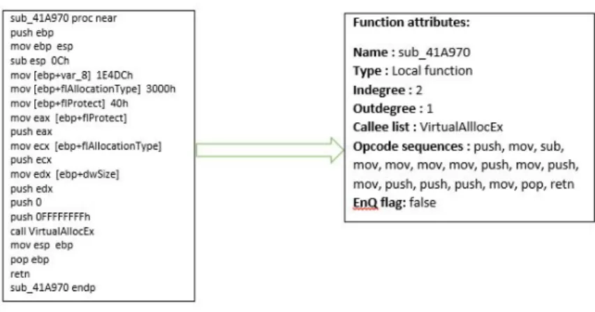
FuncQ. On building the vertices in the graph, the sub-routine name, type, callee list,
indegree, outdegree, EnQ flag status and opcode sequences are stored as shown in
Figure 1. The time complexity of this algorithm is 𝑂(|𝑉| * |𝐸|) where V is the total number of vertices and E is the total number of edges [21].
Table 1: Building the Function call graph [17]
// Input: Functions in the malware 𝐹, Output: Function call graph 𝐺𝐹
// Initializations
𝐺𝐹.𝑉 =𝜑 and 𝐺𝐹.𝐸=𝜑
EntryFuncSet=𝜑, FuncSet=𝜑, FuncQ=𝜑, VerSet=𝜑
FuncSet=SplitFuncs(𝐹)
EntryFuncSet=IdentifyEntryPointFuncs(𝑀)
FuncQ=InitQ(EntryFuncSet)
while(FuncQ is not empty)
baseVertex=Dequeue(FuncQ)
Insert baseVertex in𝐺𝐹
baseVertex.enQFlag=true
VerSet=getCallee(baseVertex)
for each vertex in VerSet if(vertex is not in FuncSet)
continue endif
headVertex=vertex
// Construct an edge between tailVertex and headVertex if(𝑒∈𝐺𝐹.𝐸) baseVertex.outDeg++ headVertex.inDeg++ else Insert headVertex in 𝐺𝐹 Insert edge 𝑒 in𝐺𝐹 endif if(headVertex.enQFlag==false)
Enqueue headVertex in FuncQ
headVertex.enQFlag=true endif next vertex end while return𝐺𝐹 end
3.3 Function Call Graph Scoring
On building the function call graph, to find the similarity score between the two malware variants we need to compare the corresponding graphs. The similarity check between the graphs would imply finding common vertices which represents the functions or sub-routines. The functions cannot be identified based on specific string or pattern search as it can be easily defeated using several obfuscation techniques. The scoring of the similarity is calculated by matching external and internal functions. The system or library functions have common function names which are of the same naming convention in all files. So, the external functions are matched based on their function names. In the local functions, to overcome challenges set by code obfuscation techniques the instructions are color coded based on its type of action.
3.3.1 Common vertices based on External Functions
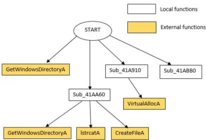
External functions generally refer to the system calls or library routine calls. The system functions are also called the atomic functions. Usually, the external functions form the leaf node in the graph with an indegree of 1 and outdegree of 0. They can be mapped using the symbolic names that are same across all executables. For example,
VirtualAllocA, GetWindowsDirectoryA, lstrcatA, CreateFileA are the external functions that forms the leaf nodes in the Zbot function call graph shown in Fig 2. Table 2 displays an algorithm that has been used to find common vertices based on external functions [17].
The external functions are taken from function call graphs of the two malware variants that are being scored for similarity 𝐺1, 𝐺2 and stored in ExtFuncSet1 and
ExtFuncSet2 respectively. The instructions in the vertices of both sets are
Figure 2: Function call graph with external functions
Table 2: Pseudocode to find common vertices using external functions [17]
// Input: Function call graph of two malware variants 𝐺1 and 𝐺2
// Output: common_vertex(𝐺1, 𝐺2)
ExtFuncSet1← External function from 𝐺1
ExtFuncSet2← External function from 𝐺2
Copy vertices from 𝐺1 into𝑈𝑠 Copy vertices from 𝐺2 into𝑉𝑠 foreach vertex 𝑈𝑠𝑖 𝜖 ExtFuncSet1 do
foreach vertex 𝑉𝑠𝑗 𝜖 ExtFuncSet2 do if(𝑈𝑠𝑖.name = 𝑉𝑠𝑗.name)
common_vertex(𝐺1, 𝐺2) ←common_vertex(𝐺1, 𝐺2) ∪ (𝑈𝑠𝑖,𝑉𝑠𝑗) Remove 𝑈𝑠𝑖 from𝑈𝑠 Remove 𝑉𝑠𝑗 from𝑉𝑠 end end end
all j vertices in ExtFuncSet2 assigned to 𝑉𝑠 and finds if both graphs have any ver-tices that call the same external function. If such a vertex is found it is stored in
common_vertex(𝐺1, 𝐺2).
3.3.2 Match local functions based on external functions similarity
If two or more external functions are found matching in a vertex, then it is considered as a similarity between the local functions that make the call to external functions. Table 3 is the pseudocode that was used to find matching local functions pair [17, 21].
Table 3: Pseudocode to find similar local functions based on external functions [17]
// Input: Function call graph 𝐺1 and 𝐺2,𝑈𝑠,𝑉𝑠,common_vertex(𝐺1, 𝐺2)
//Output: common_vertex(𝐺1, 𝐺2)
foreach vertex 𝑈𝑠𝑖 𝜖 𝑈𝑠 do foreach vertex 𝑉𝑠𝑗 𝜖 𝑉𝑠 do
if(ExtFunc(𝑈𝑠𝑖) ∩ ExtFunc(𝑉𝑠𝑗)≥ 2) then
common_vertex(𝐺1, 𝐺2) ←common_vertex(𝐺1, 𝐺2) ∪ (𝑈𝑠𝑖,𝑉𝑠𝑗) Remove 𝑈𝑠𝑖 from𝑈𝑠 Remove 𝑉𝑠𝑗 from𝑉𝑠 end end end
each of the local functions in the function call graphs 𝐺1, 𝐺2 are matched to
see if they call the same external functions. If the external functions count
ex-ceeds 2, then the function pair is considered as common vertices and added to the
common_vertex(𝐺1, 𝐺2).
3.3.3 Similarity between local functions based on opcode sequence
Finding the similarity between the local functions based on a specific pattern or signature will not be effective as it can be defeated on using simple dead code insertion itself. So, we use a unique graph coloring technique. Every vertex is vectorized based
on the occurrence and frequency of the opcodes which are classified into 15 types as shown in Table 4.
Table 4: x86 instruction classification [17]
Code Instruction Type Description
𝐶1 Data Data Transfer as mov stmt
𝐶2 Stack Stack Operations
𝐶3 Port In and out
𝐶4 Lea Destination address
trans-mit
𝐶5 Flag Flag transmit
𝐶6 Arithmetic Shift, Rotate etc.
𝐶7 Logic Bitbyte operation
𝐶8 String String operation
𝐶9 Jump Unconditional transfer
𝐶10 Branch Conditional transfer
𝐶11 Loop Loop control
𝐶12 Halt Stop instruction execution
𝐶13 Bit Bit test and bit scan
𝐶14 Processor Processor control
𝐶15 Float Floating point operation
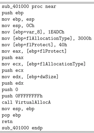
All vertices in the graph are colored base don a 15-bit variable which marks the occurrence of instructions in each color code. The variable is initialized to 0. On reading an instruction, the color code that it belongs to based on its operation is marked 1 in the corresponding bit. Another 15-bit vector stores the frequency of the corresponding color codes. Table 5 shows a sub-routine from Zbot virus and Table 6 displays the corresponding color codes and frequency vector.
Table 5: A sub-routine in Zbot virus
sub_401000 proc near push ebp
mov ebp, esp mov esp, 0Ch
mov [ebp+var_8], 1E4DCh
mov [ebp+flAllocationType], 3000h mov [ebp+flProtect], 40h
mov eax, [ebp+flProtect] push eax
mov ecx, [ebp+flAllocationType] push ecx
mov edx, [ebp+dwSize] push edx
push 0
push 0FFFFFFFFh call VirtualAllocA mov esp, ebp
pop ebp retn
sub_401000 endp
Table 6: Occurrence and Frequency color coded vector of the above Zbot sub-routine
Opcode’s C1 C2 C3 C4 C5 C6 C7 C8 C9 C10 C11 C12 C13 C14 C15
Occurrence 1 1 0 0 0 0 0 0 1 0 0 0 0 0 0
Frequency 9 7 0 0 0 0 0 0 2 0 0 0 0 0 0
The frequency vector of the two graphs are stored as 𝑋 = (𝑥1, 𝑥2, ..., 𝑥15) and 𝑌 = (𝑦1, 𝑦2, ..., 𝑦15) and the cosine similarity of them are computed as shown in
sim(𝑋, 𝑌) = ∑︀15 𝑖=1𝑥𝑖.𝑦𝑖 √︁ ∑︀15 𝑖=1𝑥2𝑖. √︁ ∑︀15 𝑖=1𝑦𝑖2 (1)
The calculated cosine similarity is checked for whether it is greater than or equal
to a threshold value of 𝛼 and we also compare the color codes of the two vertices
and if found the same the local functions are found as a common vertex match. Table 7 shows a pseudocode that is used to compute the color similarity between the vertices [17, 21].
Table 7: Pseudocode to find color similarity between two functions [17]
// Input: Functions 𝑓1 and 𝑓2
// Output: color similarity between 𝑓1 and 𝑓2
colorCode1 ← getColorSequence from𝑓1
colorCode2 ← getColorSequence from𝑓2
if(color1=color2)
freqVector1 ←getVector from 𝑓1
freqVector2 ←getVector from 𝑓2
color_sim ← compute cosine similarity between vector1 and vector2
end
return color_sim
In the pseudocode, the computation of color similarity between two functions is described. Similarly, all the functions in the malware variants are computed.The functions 𝑓1 and 𝑓2 are provided as input to calculate the cosine similarity between
the functions. The functions are first assigned a color based on the occurrence of
the instructions which are stored as colorCode1 and colorCode2 from 𝑓1 and 𝑓2.
If the color code of the two functions are found similar, then the frequency of the
corresponding instructions are stored in vectorsfreqVector1andfreqVector2. The
cosine similarity between the frequency vectors are computed using the formula(1) mentioned above. Aiming for perfection, two more criteria as the length of the opcode
sequences which refers to the number of bytes in the function and the total degree of the function which is calculated by adding the indegree (total number of times the function is called) and the outdegree (total number of times the function is called by other functions) are used for scoring. If the cosine similarity of the two frequency vectors is greater than or equal to 𝛼 and the length similarity (len_sim) is greater than or equal to 𝛽 anddegree similarity(degree_sim) is greater than or equal to 𝛾.
The length similarity is computed based on the formula (2) as shown below. The
length(𝑓1) is the number of bytes in function 𝑓1 and length(𝑓2) is the number of
bytes in function 𝑓2. The smaller value of the two is divided by the other to obtain
a value between 0 and 1.
length_sim(𝑓1, 𝑓2) = ⎧ ⎪ ⎨ ⎪ ⎩ length(𝑓1) length(𝑓2) if length(𝑓1)≤length(𝑓2) length(𝑓2) length(𝑓1) otherwise. (2)
The degree similarity is computed using the formula (3) in which thedegree(𝑓1)
is the total degree of the function𝑓1anddegree(𝑓2) is the total degree of the function 𝑓2. The degree_sim is assigned 1 if the degrees of the two functions are equal, else
the unsigned reciprocal of their differences is used.
degree_sim(𝑓1, 𝑓2) = {︃ 1 if deg(𝑓1) =deg(𝑓2) 1 |deg(𝑓1)−deg(𝑓2)| otherwise. (3)
The threshold values of 𝛼, 𝛽 and 𝛾 are set as 0.98, 0.83 and 0.5 respectively
based on previous experiments [17, 21]. Table 8 details the pseudocode to find similar function pair using the color similarity [6].
Table 8: Pseudocode to find similar local functions using color similarity [17]
// Input: Function call graph 𝐺1 and 𝐺2,𝑈𝑠,𝑉𝑠,common_vertex(𝐺1, 𝐺2)
//Output: common_vertex(𝐺1, 𝐺2) foreach vertex 𝑈𝑠𝑖 𝜖 𝑈𝑠 do foreach vertex 𝑉𝑠𝑗 𝜖 𝑉𝑠 do if(color_sim(𝑈𝑠𝑖,𝑉𝑠𝑗)≥ 𝛼 ∩ length_sim(𝑈𝑠𝑖,𝑉𝑠𝑗) ≥ 𝛽 ∩ degree_sim(𝑈𝑠𝑖,𝑉𝑠𝑗) ≥ 𝛾) then common_vertex(𝐺1, 𝐺2) ←common_vertex(𝐺1, 𝐺2) ∪ (𝑈𝑠𝑖,𝑉𝑠𝑗) Remove 𝑈𝑠𝑖 from𝑈𝑠 Remove 𝑉𝑠𝑗 from𝑉𝑠 end end end
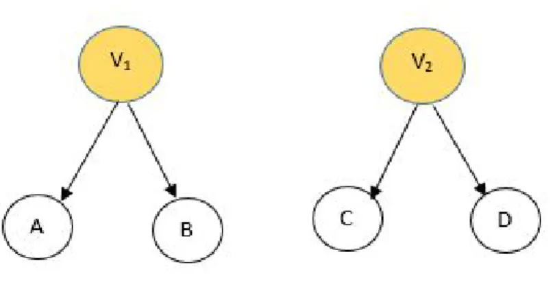
3.3.4 Similarity between local functions based on matched neighbors
Now that we have found common vertices between the two graphs based on the internal and external functions, we can further analyze based on the results. There is a high probability that two vertices are similar if their neighbors match in graph theory. So, if the predecessor or successor of a specific vertex is a common
vertex then the vertex may also be a common vertex. In Figure 3 the vertices 𝑉1
and 𝑉2 are already identified as common vertices, then its neighbors A, B and C,
D respectively are rechecked using a color_relaxed_sim to find whether they are
similar. The color_relaxed_sim is computed same as the Table 7 except that the
functions’ color codes need not match and the cosine similarity can be computed from the frequency vectors directly. Table 9 presents the pseudocode used to find similar functions based on matched successors and the same pseudocode applies for predecessors too by replacing successor(u) and successor(v) by predecessor(u) and predecessor(v) respectively. [21].
Figure 3: Successors of common vertices 𝑉1 and 𝑉2 are candidate vertices
Table 9: Pseudocode to find similar local functions based on matched successor [17]
// Input: Function call graph𝐺1 and 𝐺2,𝑈𝑠,𝑉𝑠,common_vertex(𝐺1, 𝐺2)
//Output: common_vertex(𝐺1, 𝐺2)
vertexQ← InitvertexQ(common_vertex(𝐺1, 𝐺2))
while (vertexQ is not empty)
(u,v)← vertexQ.dequeue()
foreach vertex𝑈𝑠𝑖 𝜖 successor(u) ∩𝑈𝑠 do foreach vertex𝑉𝑠𝑗 𝜖 successor(v) ∩ 𝑉𝑠 do
if(color_relaxed_sim(𝑈𝑠𝑖,𝑉𝑠𝑗)≥ 𝛿) then common_vertex(𝐺1, 𝐺2) ← common_vertex(𝐺1, 𝐺2) ∪(𝑈𝑠𝑖,𝑉𝑠𝑗) Remove 𝑈𝑠𝑖 from 𝑈𝑠 Remove 𝑉𝑠𝑗 from 𝑉𝑠 vertexQ.enqueue(𝑈𝑠𝑖,𝑉𝑠𝑗) end end end end return common_vertex(𝐺1, 𝐺2)
ThevertexQis initialized with the vertices in thecommon_vertex(𝐺1, 𝐺2). Each
vertex in the queue are dequeued one by one and the successor or predecessor of the
corresponding vertices. If the color_relaxed_sim of the successor or predecessor
are considered similar.
3.3.5 Similarity between function call graph
To compute the consolidated score of similarity between the function call graphs, the common edges are computed. The edge is the "caller-callee" relationship that
was mentioned before. If common vertices W and X share an edge in graph 𝐺1 and
common vertices Y and Z share an edge in graph𝐺2 then it is called a common edge.
The overall similarity between the two malware function call graphs are computed using Formula (4) [17, 6]:
sim(𝐺1, 𝐺2) =
2|common_edge(𝐺1, 𝐺2)| |𝐸𝑑𝑔𝑒(𝐺1)|+|𝐸𝑑𝑔𝑒(𝐺2)|
*100 (4)
in which |common_edge(𝐺1, 𝐺2)| denotes all the common edges between the two
function call graphs 𝐺1 and 𝐺2 and |𝐸𝑑𝑔𝑒(𝐺1)|+|𝐸𝑑𝑔𝑒(𝐺2)| represents the total
number of edges in graph 𝐺1 and 𝐺2. Scoring the same file should give a value of 1
and scoring a malware variant should give a value between 0 and 1 based on the level of obfuscation in which the less obfuscated would be closer to 1.
CHAPTER 4
Types of obfuscation techniques
The metamorphic virus detection has been a tough task because the virus is capable of mutating its body to an extent that no two versions of the same malware can be assigned a common signature for detection and hence are undetectable by
signature based detection [14]. This level of obfuscation in the code is achieved
by one or a combination of multiple code obfuscation techniques which are detailed below:
4.1 Instruction substitution
The instruction substitution is a simple obfuscation technique in which the com-mon instructions that have similar usage are replaced instead of the other. [15] By substituting the instruction with a similar one, the functionality of the code remains intact and the code also does not look the same as before. For example, the
instruc-tions JB (Jump if Below), JC (Jump if Carry), JNAE (Jump if Not above or Equal)
all perform the same action of setting CF (Carry Flag) as1. Using these instructions interchangeably will not affect the function of the code.
Considering this technique to impede the function call graph similarity it may not be effective, as in our detection technique, the opcodes are color coded based on functionality and used for computing the score. So, even if we substitute the instructions they will fall under the same group and will be no different from the previous code.
4.2 Register swap
Register swap is another simple technique in which the registers are swapped by not hindering the intended action of the part of the code; at the same time it forms another generation of the malware as it can evade signature based detection having altered registers all through the code. For example, the register EAX, EBX, EDX are
swapped with EBX, EDX, EAX respectively. This small change is enough to fool the
signature based detection. But if the detection method has wildcard search in place of registers it can be easily identified. [28]
Applying this technique to weaken our detection method will not fetch results as we only consider the opcodes for finding similarity and the registers are not considered for evaluation.
4.3 Subroutine ordering
In subroutine ordering, the order of the subroutines are altered in a random manner. [15, 14] Such an action will not change the effect of the code as the program with subroutines are not sequential, they call for the start address of the subroutine and thus does not hinder the functionality. For example, if a malware is composed of 8 subroutines, there are 8! ways, that is 40320 ways to mutate the malware [28].
In function call graph method, it may not be effective as we compute a graph from subroutines based on their calls and not by position.
4.4 Code transposition
Similar to the subroutine ordering, the code within the subroutine are re-ordered [15] if they do not demand computation in sequence. By shuffling the
in-structions, the signature detection can be defeated.
This technique may not be effective in our detection as the instruction sequence is not considered and only the list of opcodes are used to compute the score.
4.5 Code integration
The code integration is a more sophisticated means of obfuscating the code in which the virus on spreading the infection, attaches itself to the executable of the
host. For example, Zmist virus [6] decompiles PE (Portable Executable) of the host
file and smartly inserts the malware code by part, integrates itself and repackages the executable making it extremely hard to detect.
4.6 Dead code insertion
Dead code insertion is the most commonly used detection technique. Dead code is the piece of code that just performs meaningless actions which does not produce any results. When dead code is appended to any program it will not affect the code.
For example, the No Operation (NOP) on being inserted will not perform any action
but may tamper the signature of the malware [14, 13]. The dead code can be inserted in two ways:
1. Block morphing: In this type of morphing, a block of the dead code is inserted in the malware [15]. This may hinder the signature based detection and prove effective based on the malware. If the block added is not part of the unique part of malware extracted to make signature then it may not prove effective. 2. Random morphing: In random morphing, single or few of lines of the dead
the percentage of benign code added to malware code increases there may be a chance all the mutated codes are quite similar. The dead code used to be inserted has to be varied in each generation to fetch better results.
Dead code insertion technique used to defeat the function call graph score may result in any of the three scenarios:
1. On using block morphing, if the benign dead code is added as a block in between two subroutines or at start or end of program, the score will not be affected as the detection method only takes the subroutines and the instructions in it into consideration.
2. On using block morphing, if block of dead code is added within a subroutine, it will only affect one sub-routine and hence will not make a big difference 3. On using random morphing, if significant number of lines of dead code are
inserted in all subroutines, it may be deter or boost the scores depending on whether the code is inserted to a an already obfuscated dead coded subrou-tine (as we are dealing with metamorphic malware) or a matching sub-rousubrou-tine respectively.
The same random morphing technique when applied using external function calls as dead code is very effective in defeating the function call graph based detection.
CHAPTER 5 Experiments
In this chapter, we will be discussing on the results obtained on scoring metamor-phic malware files using function call graph analysis and few experiments on defeating the score by using code morphing.
5.1 Chosen Dataset
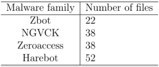
We have used NGVCK, Zbot, ZeroAccess and Harebot files to be scored. The New Generation Virus Generation Kit (NGVCK) is a metamorphic worm that has been created to defeat the Hidden Markov Model (HMM) detection technique [6] using obfuscation techniques as dead code insertion and instruction substitution. Zbot [23] and ZeroAccess [24] are trojans that infects the host system and uses stealth tech-niques to collect sensitive data. Harebot [8] is a backdoor which usually attacks the Operating system and consumes the system resources bringing down the system’s productivity. For this research, we have used 30 cygwin files for the benign dataset. Table 10 lists the number of files used in each malware family.
Table 10: Malware files
Malware family Number of files
Zbot 22
NGVCK 38
Zeroaccess 38
5.2 Receiving Operating Characteristics
Receiving Operating Characteristics(ROC) is a graphical plot that is used to measure the accuracy of detection. The ROC curve is drawn using the true positive rate(TPR) and false positive rate(FPR) by assessing several other criteria. The area under the curve (AUC) is the measured value from the plot that is used for comparing the performance from experiments. The best case of obtaining an AUC of 1.0 implies that it was a perfect classification with no false positives or false negatives. The value of the ROC may range between 0.5 and 1. Figure 4 shows the an ROC curve with an AUC value of 1.0.
Figure 4: An ROC curve with AUC = 1.0 [25]
5.3 Scoring of the files
We have implemented the function call graph detection method using Java as discussed in Chapter 3. Initially, the executable in assembly language format is pre-processed to obtain the sub-routines of the specific file. After the first set of trial experiments in NGVCK family as shown in Fig 5, we had to adjust the threshold values of 𝛼, 𝛽 and 𝛾 as 0.80, 0.5 and 0.5 respectively as it produced more accurate results for the chosen dataset.
0 0.1 0.2 0.3 0.4 0.5 0.6 0.7 0.8 0.9 1 0 0.1 0.2 0.3 0.4 0.5 0.6 0.7 0.8 0.9 1
False Positive Rate
T rue P ositiv e Rate 𝛼-0.98,𝛽-0.83,𝛾-0.5 𝛼-0.8,𝛽-0.5,𝛾-0.5
Figure 5: NGVCK ROC curve with change in threshold values
5.3.1 NGVCK files
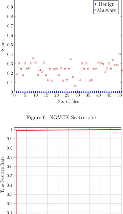
We scored the NGVCK files using our detection method and was able to classify the benign files and malware variants. On scoring the malware files with benign files, most of the scores were 0.0 denoting no similarity between the files and the maximum score was 0.044 whereas scoring the malware variants within themselves most of the scores were above 0.2.
Figure 6 shows the scatter plot that clearly classifies the files and Figure 7 shows an ROC curve based on the scores obtained which gives an AUC of 0.99 which is good as it is very close to 1.0.
0 5 10 15 20 25 30 35 40 45 50 0 0.1 0.2 0.3 0.4 0.5 0.6 0.7 0.8 0.9 1 No. of files Scores Benign Malware Figure 6: NGVCK Scatterplot 0 0.1 0.2 0.3 0.4 0.5 0.6 0.7 0.8 0.9 1 0 0.1 0.2 0.3 0.4 0.5 0.6 0.7 0.8 0.9 1
False Positive Rate
T rue P ositiv e Rate
5.3.2 Zbot files
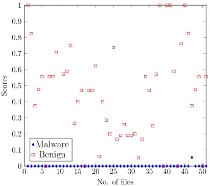
The Zbot files were also scored using the function call graph implementation and successfully classified the benign and malware files. The malware variants when scoring within themselves gave high values and on scoring with benign files they showed no similarity by scoring 0.0 for most files.
Figure 8 displays the differentiation between benign and malware files and Fig-ure 9 shows the ROC curve which are plotted using the scores and it provides an AUC of 0.96. 0 5 10 15 20 25 30 35 40 45 50 0 0.1 0.2 0.3 0.4 0.5 0.6 0.7 0.8 0.9 1 No. of files Scores Malware Benign
0 0.1 0.2 0.3 0.4 0.5 0.6 0.7 0.8 0.9 1 0 0.1 0.2 0.3 0.4 0.5 0.6 0.7 0.8 0.9 1
False Positive Rate
T rue P ositiv e Rate
5.3.3 ZeroAccess files
On scoring the ZeroAccess files using our detection method, we found that it failed to get classified as clear as the previous families. The benign files when scored with malware files had the maximum score of 0.03 and on scoring with its malware variants scores an average of 0.07.
Figure 10 shows the scatter plot of the ZeroAccess files in which the benign and malware files seem to score similar except for a few outliers and Figure 11 shows an ROC curve of the ZeroAccess files with an AUC of 0.77.
0 5 10 15 20 25 30 35 40 45 50 0 0.1 0.2 0.3 0.4 0.5 0.6 0.7 0.8 0.9 1 No. of files Scores Malware Benign
Figure 10: ZeroAccess Scatterplot
5.3.4 Harebot files
On scoring the Harebot files, the results were relatively worse than the ZeroAccess family. Most of the benign files and malware files score the same and there is no distinct classification between the two files.
0 0.1 0.2 0.3 0.4 0.5 0.6 0.7 0.8 0.9 1 0 0.1 0.2 0.3 0.4 0.5 0.6 0.7 0.8 0.9 1
False Positive Rate
T rue P ositiv e Rate
Figure 11: ZeroAccess ROC Curve
Figure 12 shows the scatter plot in which it is evident that the benign and malware files are not distinctly clear and Figure 13 shows an the ROC plotted with the results fetching an AUC of 0.60.
5.3.5 Analysis of scores
In the four families, NGVCK and Zbot have scored well by using function call graph analysis. But, function call graph detection failed to classify the malwares in ZeroAccess and Harebot families. On having a closer look at the files, it was evident that in cases when two files which had big difference in their file sizes did not score well. In Chapter 3, when computing similarity between the graphs using Formula (4) as the common edges are not normalized with respect to the total number of edges in each graph they fail to score well. To clarify the assumption we scored the ZeroAccess and Harebot files in sets classified based on file size.
0 5 10 15 20 25 30 35 40 45 50 0 0.1 0.2 0.3 0.4 0.5 0.6 0.7 0.8 0.9 1 No. of files Scores Malware Benign
Figure 12: Harebot Scatterplot
0 0.1 0.2 0.3 0.4 0.5 0.6 0.7 0.8 0.9 1 0 0.1 0.2 0.3 0.4 0.5 0.6 0.7 0.8 0.9 1
False Positive Rate
T rue P ositiv e Rate
5.4 Scoring the files in sets
The files are partitioned in sets based on file sizes and scored using the function call graph analysis.
5.4.1 ZeroAccess family
On scoring the 120 ZeroAccess files as sets, the ZeroAccess family scored well. In fact, it achieved a perfect AUC of 1.0 in one of the sets. Table 11 shows the details of the files in the sets and the corresponding AUC values. Figure 14 shows the ROC curves of the sets in the ZeroAccess family.
Table 11: Zero Access files set
No. of files Filesize Range AUC Values
Set 1 20 25 - 30 KB 0.91
Set 2 40 31 - 40 KB 0.74
Set 3 40 110 - 112 KB 0.96
Set 4 20 114 - 128 KB 1.0
5.4.2 Harebot family
On scoring 40 Harebot files in two sets, though there is a substantial increase in the AUC values the classification is not discrete. On further analysis on the files, we found that the reason for low scores in Harebot was because it had only a couple of external functions in each program. Since atleast two external functions from same sub-routine has to match to be considered common vertex, Harebot may not have any similarity in the external functions attribute. Table 12 shows the details of the files in the sets and the corresponding AUC values. Figure 15 shows the ROC curves of the sets in the ZeroAccess family.
0 0.1 0.2 0.3 0.4 0.5 0.6 0.7 0.8 0.9 1 0 0.1 0.2 0.3 0.4 0.5 0.6 0.7 0.8 0.9 1
False Positive Rate
T rue P ositiv e Rate Set 1 Set 2 Set 3 Set 4
Figure 14: ZeroAccess ROC curve of the sets Table 12: Harebot file sets
No. of files Filesize Range AUC Values
Set 1 20 7 - 11 KB 0.74
Set 2 20 13 - 31 KB 0.62
5.5 Defeating the score
In this section, we have defeated the function call graph scoring method. The code obfuscation used to morph the malware is dead code insertion. As discussed in Chapter 4, block morphing will fail to defeat the method as it only affects one sub-routine. We have used external functions as dead code and randomly inserted it as chunks of code in all subroutines.
0 0.1 0.2 0.3 0.4 0.5 0.6 0.7 0.8 0.9 1 0 0.1 0.2 0.3 0.4 0.5 0.6 0.7 0.8 0.9 1
False Positive Rate
T rue P ositiv e Rate Set 1 Set 2
Figure 15: Harebot ROC curve of the sets
5.5.1 NGVCK family
Starting from 15% random morphing, we can see the effect in the AUC values. Figure 16 shows the ROC curves starting from 5% to 40% in which there is a significant change from 10% to 15% ˙Since there is a hill climb behavior in 35% we plotted the
morphed values from 10% to 200% in which the score gradually increases. This
indicates that a threshold of 15% to 35% should be set for morphing to defeat the NGVCK score. Figure 17 clearly visualizes the necessity to set a threshold value for morphing.
5.5.2 Zbot family
Similar to the NGVCK family, Zbot also has low AUC values starting from 15% and the pattern continues until 35% after which a gradual increase is to be noted. The difference in the scores from 10% to 15% is graphically depicted using ROC curves in
Figure 16: NGVCK Morphed ROC Curve 0 0.1 0.2 0.3 0.4 0.5 0.6 0.7 0.8 0.9 1 0 0.1 0.2 0.3 0.4 0.5 0.6 0.7 0.8 0.9 1
False Positive Rate
T rue P ositiv e Rate 5% morphing 10% morphing 15% morphing 20% morphing 25% morphing 30% morphing 35% morphing 40% morphing Figure 18. 5.5.3 Consolidated results
The consolidated results from the external function dead code random morphing is displayed in Table 13. Both NGVCK and Zbot files starting 15% show promising results. Notably, as the morphing % increases the malware variants are found similar within themselves. Hence, a threshold must be set on the level of morphing to defeat the method consistently.
5.6 Scoring files on a larger number of files
To find whether the results are consistent, the function call graph scoring is experimented on more no. of files. Table 14 shows the malware families and the
Figure 17: NGVCK Morphed 10% - 200% 10 20 30 40 50 60 70 80 90 100110120130140150160170180190 0.65 0.7 0.75 0.8 0.85 0.9 0.95 Morphing% A UC V alues
Table 13: AUC curve results for morphed NGVCK and Zbot files
AUC Morphing NGVCK Zbot 0% 0.99 0.96 5% 0.99 0.96 10% 0.98 0.93 15% 0.75 0.84 20% 0.64 0.87 25% 0.65 0.84 30% 0.62 0.83 35% 0.65 0.84 40% 0.67 0.83
0 0.1 0.2 0.3 0.4 0.5 0.6 0.7 0.8 0.9 1 0 0.1 0.2 0.3 0.4 0.5 0.6 0.7 0.8 0.9 1
False Positive Rate
T rue P ositiv e Rate 5% morphing 10% morphing 15% morphing 20% morphing 25% morphing 30% morphing 35% morphing 40% morphing
Figure 18: Zbot Morphed ROC Curve
number of files used for this experiment.
Table 14: Number of files used in each family
Malware family Number of files
Zbot 100
NGVCK 100
Zeroaccess 100
5.6.1 NGVCK family
On scoring the larger dataset, the AUC values are lower which maybe because of a few outliers in the total files used. Figure 19 shows an AUC of 0.94 which is still a good score and classifies most malwares from the files.
0 0.1 0.2 0.3 0.4 0.5 0.6 0.7 0.8 0.9 1 0 0.1 0.2 0.3 0.4 0.5 0.6 0.7 0.8 0.9 1
False Positive Rate
T rue P ositiv e Rate
Figure 19: NGVCK ROC Curve (100 files)
5.6.2 Zbot family
The Zbot family seem to have a setback in the AUC value. As shown in Figure 20 has an AUC of 0.8 which fails to classify the malware effectively. At a closer look on the files used, similar to ZeroAccess it has a larger difference in the file sizes used. By dividing it into sets based on filesize, we can have a clearer picture of the overall score for Zbot family. Table 15 shows the details about each set and Figure 21 shows the AUC values of the sets.
Table 15: Zbot sets
No. of files Filesize Range AUC Values
Set 1 30 4 KB 0.84
Set 2 60 5 KB 0.72
Set 3 20 6 - 8 KB 0.96
0 0.1 0.2 0.3 0.4 0.5 0.6 0.7 0.8 0.9 1 0 0.1 0.2 0.3 0.4 0.5 0.6 0.7 0.8 0.9 1
False Positive Rate
T rue P ositiv e Rate
Figure 20: Zbot ROC Curve (100 files)
0 0.1 0.2 0.3 0.4 0.5 0.6 0.7 0.8 0.9 1 0 0.1 0.2 0.3 0.4 0.5 0.6 0.7 0.8 0.9 1
False Positive Rate
T rue P ositiv e Rate
5.6.3 ZeroAccess family
The score of the ZeroAccess family is consistent with the previous experiment. Figure 22 shows the AUC value of 0.75 in the Zero Access ROC curve.
0 0.1 0.2 0.3 0.4 0.5 0.6 0.7 0.8 0.9 1 0 0.1 0.2 0.3 0.4 0.5 0.6 0.7 0.8 0.9 1
False Positive Rate
T rue P ositiv e Rate
CHAPTER 6
Conclusion and Future Work
The main goal of our project was to study the function call graph analysis [6, 17, 21], implement and score it on metamorphic malware families and defeat the score to understand how the detection method can be made more effective and efficient. The function call graph analysis scores the metamorphic malware based on similar external functions, local functions that have similar external functions, cosine similarity based on frequency of opcodes which are classified and color coded based on the purpose of the instructions and matching neighbors of similar local functions. Additionally, the length of the functions and degree similarity are also added as thresholds to make the detection effective. From all the above comparisons, the common vertices between the function call graphs of the two malware variant is found. Using these common vertices, the total number of common edges between the vertices of the graphs are found and used to score the malwares.
We scored four malware families: NGVCK, Zbot, ZeroAccess and Harebot to analyze how the detection technique is effective in these families. The NGVCK and Zbot detected the malware and classified them by scoring higher than the benign files. But the ZeroAccess and Harebot families were not very successful in detecting the malwares. We also tried to defeat the NGVCK and Zbot scores using random block morphing and achieved considerable success in it.
For future work, these experiments can be implemented in comparison of different
threshold parameters 𝛼, 𝛽 and 𝛾, as some malware families perform well at higher
external functions similarity [29], opcode graph similarity [20] and the function call graph similarity [17] can be incorporated to build a hybrid robust detection technique that can overcome all the limitations of the detection methods. The common vertices by external functions happen to be the most contributing factor in the score which can be exploited by random morphing of benign external function calls. The external function based match has to be normalized based on total number of external function
calls. The function call graph detection technique is more effective in files with
same number of sub-routines. On considering two malware variants, in which one is obfuscated extensively by adding dead code the function call graph method fails to identify one file as the subset of other which implies it is similar. To rectify this flaw, the common edges need to be normalized not just by the total number of edges in both graphs but by total number of edges in each graph.
LIST OF REFERENCES
[1] S. Alam, I. Trore, I. Sogukpinar, Annotated Control Flow Graph for
Metamor-phic Malware Detection,Security in Computer Systems and Networks, The
Com-puter Journal, 2014
[2] J. Aycock, Computer Viruses and Malware, Advances in Information Security,
Springer-Verlag, New York, 2006
[3] A. P. Bradley, The Use of the Area Under the ROC Curve in the Evaluation
of Machine Learning Algorithms, Journal Pattern Recognition, 30(7):1145–1159,
1997
[4] M. Christodorescu and S. Jha, Static analysis of executables to detect malicious
patterns, Proceedings of 12th conference of USENIX Security Symposium,
Vol-ume 12, Washington DC ,2003
[5] Common Malware Types: Cybersecurity 101,
https://www.veracode.com/blog/2012/10/common-malware-types-cybersecurity-101 (accessed December 17, 2015)
[6] P. Deshpande, Metamorphic Detection Using Function Call Graph Analysis, Master’s report, Department of Computer Science, San Jose State University, 2013,
http://scholarworks.sjsu.edu/etd_projects/336
[7] Fortinet 2014 Threat Landscape Report,
http://www.fortinet.com/resource_center/whitepapers/threat-landscape-report-2014.html (accessed December 17, 2015)
[8] Harebot. M
http://www.pandasecurity.com/homeusers/security-info/220319/ Harebot.M (accessed December 17, 2015)
[9] N. Idika and A. Mathur, A Survey of Malware Detection Techniques, 2007
http://www.serc.net/systems/files/SERC-TR-286.pdf (accessed December 17, 2015)
[10] A. Karnik, S. Goswami and R. Guha, Detecting Obfuscated Viruses Using Cosine
Similarity Analysis, Modelling and Simulation, First Asia International
[11] C. J. Keesey, How Extensive is Malware in Today’s Business World? The Realities, and the Best Protection,
https://www.linkedin.com/pulse/how-extensive-malware-todays-business-world-realities-keesey?trkSplashRedir=true&forceNoSplash=
true (accessed December 17, 2015)
[12] C. Kingsford, Graph Traversals,
http://www.cs.cmu.edu/~ckingsf/class/02713-s13/lectures/lec07-dfsbfs.pdf (accessed December 17, 2015)
[13] E. Konstantinou and S. Wolthusen, Metamorphic Virus: Analysis and Detection, Technical Report,
http://www.ma.rhul.ac.uk/static/techrep/2008/RHUL-MA-2008-02.pdf
(accessed December 17, 2015)
[14] A. Lakhotia, Are Metamorphic Viruses Really Invincible?, Virus Bulletin, December 2004,
http://www.iscas2007.org/~arun/papers/invincible-complete.pdf
(accessed December 17, 2015)
[15] D. Lin and M. Stamp, Hunting for undetectable metamorphic viruses, Journal
in Computer Virology, 7(3):201–214, Aug 2011 [16] McAfee Labs Threats Report, February 2015,
http://www.mcafee.com/us/resources/reports/rp-quarterly-threat-q4-2014.pdf (accessed December 17, 2015)
[17] X. Ming, W. Lingfei, Q. Shuhui, X. Jian, Z. Haiping, R. Yizhi and Z. Ning, A similarity metric method of obfuscated malware using function-call graph,
Journal in Computer Virology and Hacking Techniques, 9(1):35–47, 2013
[18] C. Nachenberg, Computer Virus Co-evolution, 1997, Communications of the
ACM, 40(1):46–51, Jan 1997
[19] Norton by Symantec, Bot and Botnets - A Growing Threat,
http://us.norton.com/botnet/ (accessed December 17, 2015)
[20] N. Runwal, R. Low and M. Stamp, Opcode Graph Similarity and Metamorphic
Detection, Journal in Computer Virology, 8(2):37–52, May 2012
[21] S. Shang, N. Zheng, J. Xu, M. Xu adn H. Zhang, Detecting malware variants via
function-call graph similarity, Malicious and Unwanted Software (MALWARE),
2010 5th International Conference, IEEE, pp. 113–120, 2010
[22] A. Sharma and S. K. Sahay, Evolution and Detection of Polymorphic and
Meta-morphic Malwares: A Survey, International Journal of Computer Applications,
[23] Trojan.Zbot http://www.symantec.com/security_response/writeup.jsp?docid=2010-011016-3514-99 (accessed December 17, 2015) [24] Trojan.ZeroAccess http://www.symantec.com/security_response/writeup.jsp?docid=2011-071314-0410-99 (accessed December 17, 2015)
[25] S. Vemparala, Malware Detection Using Dynamic Analysis, Master’s report, De-partment of Computer Science, San Jose State University, 2015,
http://scholarworks.sjsu.edu/etd_projects/403 (accessed December 17, 2015)
[26] P. Vinod, V. Laxmi, M. S. Gaur, Survey on Malware Detection Methods,Hack.in
2009,3rd Hackers’ Workshop on Computer and internet Security, pp. 74–79, March 2009
[27] What is Malware, and How to Protect Against It?,
http://usa.kaspersky.com/internet-security-center/internet-safety/what-is-malware-and-how-to-protect-against-it (accessed December 17, 2015)
[28] I. You and K. Yim, Malware Obfuscation Techniques: A Brief Survey,
Inter-national Conference on Broadband, Wireless Computing, Communication and Applications, pp. 297–300, 2010
[29] Q. Zhang and D. S. Reeves, MetaAware: Identifying Metamorphic Malware,
Proceedings of the Annual Computer Security Applications Conference (ACSAC), 2007.
![Table 4: x86 instruction classification [17]](https://thumb-us.123doks.com/thumbv2/123dok_us/10012915.2493643/27.918.215.756.259.645/table-x-instruction-classification.webp)
![Figure 4: An ROC curve with AUC = 1.0 [25]](https://thumb-us.123doks.com/thumbv2/123dok_us/10012915.2493643/39.918.270.680.471.712/figure-roc-curve-auc.webp)